OdeFactory User Guide
OdeFactory User Guide
(click here to get a free copy of OdeFactory 2.1, Mac version 1/29/19)
back to TOC
(0) Preface
- Dynamical systems, defined by vector fields of dimension four or less, can be created using OdeFactory. The systems can be studied as ordinary differential equations and as discrete iteration maps. Whether you think of the underlying mathematics as that of odes or discrete iterations, OdeFactory can generate appropriate phase space images, or "views," of the dynamical systems.
The vector fields themselves are t-advancing maps from Rn to Rn defined by lists of closed-form mathematical expressions (lists of algorithms in computer terminology) consisting of:
- 24 elementary functions: exp, sqrt, sin, cos, tan, asin, acos, atan, ln, log, sinh, cosh, tanh, abs, ceil, floor, max, min, round, step, sgn, pm, pulse and random (the first 19 are defined in the java.lang.Math class, step through random are defined in OdeFactory),
- left and right parentheses: (, ),
- 2 constants: pi and e,
- 4 generic state variables: x, y, z and w,
- the "time" advancing variable: t,
- 6 arithmetic operators: +, -, *, /, % and ^,
- 14 user defined parameters designated by single lower case letters other than x, y, z, w, t, e, i, j, l, o, u and v,
- user defined "functions" designated by upper case letters, consisting of closed-form mathematical expressions containing elementary functions, left and right parentheses, constants, state variables, time, arithmetic operators and parameters.
The "t-advancing" is implemented using three related, but fundamentally different, primary viewing algorithms. They are called the "Ode" view, the "IMap" view and the "EMap" view.
The Ode View
Traditionally, solving an "ordinary differential equation" means that given an equation involving an unknown function of time, say x(t), and some of its derivatives, the goal is to find an arithmetic expression for x(t) that satisfies the differential equation. Knowing x(t) enables you to predict the future based on some starting knowledge (initial conditions) of the present. The equation is often thought of as a "Law of Nature," or in contemporary parlance, "a model."
For example, Newton's first law of motion "F = ma," applied to the motion of a mass on a spring is
F = -k*x = m*a = m*x'' where
x is the distance of the mass from equilibrium, -k*x is the restoring force and x'' is the acceleration. Setting k = m = 1 and rewriting Newton's law as "ma = F," gives the single 2nd order ode
x'' = -x.
The solution, for the initial position x(0) and the initial velocity x'(0), is
x(t) = x(0)*cos(t)+x'(0)*sin(t).
Another way to view the problem is as follows. Let
y = x', then
y' = x'' = -x and
we can replace the 2nd order ode x'' = -x with two 1st order odes
x' = dx/dt = y,
y' = dy/dt = -x.
You can think of the 2D 1st order system of odes as being defined by the vector field
v(x,y) = (y,-x).
In OdeFactory, in the Ode view, the vector field is thought of as generating a flow or continuous motion in a phase space, that is, as a t-advancing map between regions in the phase space. No "equations" for "dx/dt" and "dy/dt" are being "solved" for x(t) and y(t).
In fact arithmetic expressions for x(t) and y(t) can only be found for rather simple vector fields. When you consider that the expressions defining the vector fields are composed of a rather small number of named "elementary" functions, and a few arithmetic operators, it is not surprising that the solution functions may define curves that cannot be written in terms of elementary functions and arithmetic operators. There are infinitely many more curves than there are names of curves. So - "solving" differential equations is a hopeless 17th century dream of Mathematicians.
In OdeFactory, there are really no "equations." No functions x(t) and y(t) are being solved for in the sense of finding functions that satisfy dx/dt = f(t,x(t),y(t)), dy/dt = g(t,x(t),y(t)). In the program the vector fields are represented by ordered lists of text strings that define closed-form mathematical expressions in terms of built-in Java arithmetic operators and the standard elementary math functions. You could also think of the vector field simply as a lists of simple (from the computer's point of view) algorithms. To OdeFactory the "equations" notation is just a superfluous decoration.
The various subviews of the Ode view are implemented using the RK4 stepping algorithm where the discrete "time" step is on the order of 0.01 units. The RK4 algorithm is used because it efficiently generates good approximate (good to the 227 PPI resolution of contemporary "Retina" displays) solution curves for almost all systems of odes.
In the case of 2D vector fields, the Ode subviews are:
- the color-coded view of the vector field itself,
- the trajectories and/or animated flow
view in R2 and in R2+,
- the 3D solution curves view in the extended phase space R3 plus the dependent (x,y), (t,x) and (t,y) projections, and
- independent time series views of x(t) and y(t) in the (t,x) and (t,y) planes.
Not all of these subviews are appropriate for 1D, 3D and 4D systems.
The IMap View
In the IMap view, vector fields are thought of as defining iteration maps (systems of 1st order recurrence relations) and the various subviews are generated using a simple stepping algorithm where the "time" step can be thought of as 1 time unit or as 1 iteration step. What are called initial conditions and trajectories in the Ode view are called seeds and orbits respectively in the IMap view.
In Math notation, a 2D iteration would be defined by a systems of 1st order recurrence relations containing subscripted state variables, for example:
x(n+1) = f(x(n),y(n)),
y(n+1) = g(x(n),y(n)).
Solving the systems of 1st order recurrence relations in closed form means finding functions X(n) and Y(n) such that:
X(n) = x(n) and Y(n) = y(n).
Finding functions X and Y is generally not possible, however the recurrence relations are just lists of algorithms where the right hand sides can be used to compute the left hand sides starting with a seed value (x(0),y(0)) = (a,b).
In Java notation, the equals sign designates the replacement operator so subscripted variables are not used and the 2D iteration is written as:
x = f(x,y),
y = g(x,y).
To avoid confusion between the use of the symbol "=" in the Math context and the computer context, I will use "<-" to stand for computer iteration and write the iteration symbolically as:
x <- f(x,y),
y <- g(x,y).
You can read the symbol "<-" as "gets" or as "is replaced by." You can think of the iteration of the system as being "atomic," meaning taking place all at once, but in Java code, the iteration is really:
xNew = f(x,y); // xNew gets f of old x and old y
y = g(x,y); // y gets g of old x and old y
x = xNew; // x gets xNew
In the case of 2D vector fields, the IMap subviews are:
- a color-coded view of the points in each orbit,
- a color-coded view of the lines between the points in each orbit,
- an animated flow of the last orbit defined,
- the 3D orbits view in the extended phase space R3 plus the dependent (x,y), (t,x) and (t,y) projections, and
- independent time series views of x(t) and y(t) in the (t,x) and (t,y) planes.
For IMaps, t is a non-negative integer. IMaps have a future but no past. Not all of these subviews are appropriate for 1D, 3D and 4D systems.
The EMap View
The EMap view is a variation of the IMap view that uses the escape time algorithm. Each pixel in the display area is visited and the pixel is given a color which depends on how many steps, starting with step 1, it takes for an orbit starting at the pixel to "escape."
In OdeFactory the escape time algorithm can be applied in the (x,y) view of a 2D or 4D system. The EMap view applies to both smooth and nonsmooth vector fields which may have several or no parameters. Smooth vector fields often give floral EMaps while nonsmooth vector fields give more geometric EMaps.
For example, in the case of the 2D Mandelbrot iteration:
x <- x^2-y^2+p, y <- 2*x*y+q,
applying the algorithm in the phase space, (x,y), gives a Julia set for each choice of parameters (p,q).
For the 4D companion system:
x <- x, y <- y, z <- z^2-w^2+x, w <- 2*z*w+y,
applying the algorithm in the (x,y) view, gives the Mandelbrot set.
The default number of colors used by OdeFactory in an EMap is 100 but it can be toggled to 512 using "Show EMap w/Max Detail" on the "Settings" menu. If you want a system in a gallery to open in the EMap view with maximum detail use EMapMax or EMapMaxCTn, with n = 0, 2, . . . 10, in the system's name.
"To escape" means that the iteration point leaves a circle of radius sqrt(50) centered at the origin before the 100th (or 512th) iteration. The value 50, is called the bailout value. Points that escape fast, that is in a small number of steps, are given a color on the right end of a color scale and points that escape slow are given a color on the left end of the color scale. Points that do not escape in 100 (or 512) iterations are colored black. The black regions are called basins of attraction.
The size of the color table, the colors in the color table, the bailout value and the resolution of the display all affect the details of an EMap image so it is generally not possible to tell if two images created by different computer programs are the same unless you know the details of how the images were computed.
back to TOC
(1) Overview of OdeFactory
- OdeFactory is a small, free, web-integrated, easy to use interactive development environment that can be used to create parameterized vector fields of dimension 4 or less. Originally the vector fields were used to define ordinary differential equations of order 4 or less but the program has been extended to include discrete 1D and 2D maps. It can now be used to study the qualitative features of vector fields, odes and maps as they relate to each other.
- The program has been designed for use by both students and instructors in introductory college ode and/or dynamical systems courses. Students with notebook computers can actively participate in class by entering odes or maps and investigate their properties as instructors lecture on the theory of the systems. Instructors can create examples and demonstrate live versions of odes and maps during their lectures. Instructors can post galleries of odes and maps discussed in class, together with associated problem sets, on the web. Instructors and students can exchange galleries as small email attachments.
- In addition to providing an interactive supplement to traditional ode textbooks, OdeFactory can also be used in conjunction with ode video courses and/or text based ode courses on the web and with distance-learning ode courses. See the Help Menu for links to video and text based ode courses on the web.
- In OdeFactory, the differential equations are entered in a simple math/computer expression syntax. Solution curves are generated by clicking or dragging in the graphics area. No knowledge of computer programming is required. Equations, parameter values, solution curves and any user written comments concerning each system being studied can be saved, in the form of a "gallery."
In addition to the usual drawing of solution curves, OdeFactory enables you to:
- do animations of the motion associated with dynamical systems,
- find and show separatrices for 2D systems,
- find and show limit cycles for 2D systems,
- view slope fields for 1D systems and vector fields for 2D systems,
- view the Poincaré map (PMap) for 2D systems with sin(. . .t. . .) or cos(. . .t. . .) driving terms,
- show 3D views of solution curves,
- study 1D and 2D discrete iteration maps and 2D Julia sets (fractals) and
- do real-time manipulation of control parameters in all views.
OdeFactory can be used to create, edit and investigate:
- general first order 1D to 4D systems,
- single odes, in normal form, of order 1 to 4,
- quasiHamiltonian 2D systems and
- algebraically generated flows (AGFs).
In the case of a given first order system, or an ode in normal form, the problem is to find the general dynamic features resulting from the system. If you instead want to study a 2D system with some specify predefined features, you can build the system as a quasiHamiltonian system or as an AGF.
The following is a discuss of the four ways in which odes can be entered into the program.
General First Order Systems of Odes Defined by a Vector Field
- A general nonautonomous first order system of odes has the form:
dx(t)/dt = v(t,x,p), x ∈ U = an open domain of Rn
where x = (x1, ... ,xn) and v is a vector valued function of the scaler t, the vector x and the set of parameters p. The scaler t is generally called time and the function v is called the vector field (sometimes called the velocity field). U is called the state space or the phase space and the vector p containing p is called the parameter space. All odes can be written in the above form. The system of odes is called the evolution equation or evolution law for a dynamical system.
Since n is at most 4 in OdeFactory, subscripts are dispensed with in favor of the simple variable names x, y, z and w. The system of odes then has the form:
dx/dt = f(t,x,y,z,w,p),
dy/dt = g(t,x,y,z,w,p),
dz/dt = h(t,x,y,z,w,p),
dw/dt = k(t,x,y,z,w,p)
The right hand side functions may include the standard math functions: abs, sqrt, sin, cos, tan, asin, acos, atan, ln, log, sinh, cosh, tanh, exp, step, sgn, max and min, as well as various parameters. The engineering function step(x), is 0 if x < 0 and 1 if x >= 0. You can right-shift the unit "step" to x = d by using step(x-d). The parameter d is called the delay. The constants e and pi may also be used. Parameter names are restricted to single lower case letters other than the reserved variable names x, y, z, w, t the constant name e and the letters i, j, l, o, u and v. User defined function names are restricted to single upper case letters. Computer syntax must be used for the right hand side functions. Arithmetic operators are: +, -, *, /, % and ^. The operator ^ is used for exponentiation and the operator % is the Java remainder, or modulo, operator. See Q&A 41 for more regarding the % operator.
For example, we could define a 1st order system of two odes by entering expressions for the first two right hand side functions, control parameters a and b, and user defined functions P and Q as follows:
- Note that the state variables, x and y as shown above, must be entered simply as coordinate names x and y, not as functions x(t) and y(t). The form of a parameter list is: name = number; ... name = number where the numbers are Java integers or doubles (not expressions) and the form of a user defined function list is: name = expression; ... name = expression where the expressions may contain: variable names, standard functions, arithmetic operators and/or user defined parameters - but not other user defined functions.
Note that the user defined "functions" are not functions in the mathematical sense in that they do not take arguments. They act more like the macros that are often used by C programmers. Just before the strings defining the vector field are converted from infix to postfix notation, any names of user defined functions used in the strings are replaced by the strings defining the functions.
Single Odes in Normal Form
- Ordinary differential equations of order n are often written in Math textbooks in normal form:
y(n) = F(x,y,y', ... , y(n-1)),
where x is the independent variable and y is the dependent variable. In OdeFactory, we call this the "y(x) form." For an n-th order ode or a 1st order system of n odes, the general solution y(x) will contain n arbitrary parameters that are fixed once n initial conditions, ICs for short, are imposed. Traditionally the closed form solution, if it can be found (try WolframAlpha, WA for short), together with the ICs, can be used to find a particular solution y(x) which in turn can be used to plot the particular solution curve.
- Particular solution curves for odes in the y(x) form, of order 4 or less, can be plotted directly without finding the general closed form solution using OdeFactory. The trick is to turn the y(x) form of the n-th order ode into an equivalent system of n 1st order odes as follows.
- First rename the independent variable x as t and the dependent variable y as x in the function F. The ode then becomes:
x'''' = F(t,x,x',x'',x''').
Introducing new variables y = x', z = x'' and w = x''', the original 4th order ode becomes the following 1st order system of 4 odes:
dx/dt = y
dy/dt = z
dz/dt = w
dw/dt = F(t,x,y,z,w)
- This translation process from a single n-th order ode in the y(x) form to a first order system of n odes is straightforward, but can be tedious, consequently OdeFactory has been programmed to generate the 1st order system for you if you simply enter:
y'''' = F(x,y,y',y'',y''')
in the "y(x) form" field in the "Define a General 1st Order Ode System" dialog window.
- For example, given the 3rd order ode y''' - y'' +sin(y') -x*y = 0, simply enter y''' = x*y -sin(y') + y'' and click the "Update Sys" button:
to generate the 1st order system for dx/dt, dy/dt and dz/dt.
- ICs in the normal form coordinates, (x,y,y',y'',y'''), correspond to ICs in the 1st order system form coordinates, (t,x,y,z,w), as follows:
y(a) = b1 ↔ x(a) = b1
y'(a) = b2 ↔ y(a) = b2
y''(a) = b3 ↔ z(a) = b3
y'''(a) = b4 ↔ w(a) = b4
so the ICs vector, (a,b1,b2,b3,b4), is the same in both coordinate systems.
- When plotting solution curves in OdeFactory for odes entered in the y(x) form, it helps to think of the (t,x,y,z,w) buttons at the bottom of the graphics area as (x,y,y',y'',y''') buttons. So - if you have a system that corresponds to a single ode in normal form with solution y(x),
y(x) ↔ x(t) in the (t,x,y)/(t,x) view
y'(x) ↔ y(t) in the (t,x,y)/(t,y) view
y''(x) ↔ z(t) in the (t,z,w)/(t,z) view
y'''(x) ↔ w(t) in the (t,z,w)/(t,w) view
assuming that you use the same ICs in the (x,y) and (z,w) views.
QuasiHamiltonian 2D Systems Defined by Curves in R2
- By a quasiHamiltonian 2D system I mean a system generated by a list of as many as ten curves (called generators) in R2 as follows:
- let H = P(x,y)*Q(x,y)*R(x,y)*···
- set dx/dt = a*Py*Q*R+b*P*Qy*R+c*P*Q*Ry+···) and
- set dy/dt = -(a*Px*Q*R+b*P*Qx*R+c*P*Q*Rx+···)
where Px, Py, ··· indicates partial derivatives with respect to x and y.
Only when all of the coefficients (control parameters) are equal to one is the system a Hamiltonian system. It then reduces to:
dx/dt = Hy, dy/dt = - Hx.
The generators contain trajectories of the system for all values of the control parameters. If you enter the generators in the "user fns:" field of the "Define a General 1st Order Ode System" window, and leave the other fields (except possibly the "params:" field) completely empty (not even any blanks), when you click the "Update Eqns, Params &/or Fns" button, OdeFactory will generate dx/dt, dy/dt and the parameter list for you. You can then start some trajectories and use the "Adj Ctrl Params..." button to explore the system.
I you want to include some of your own parameters in your generator functions, for example:
P = y-a*x^2; Q = y-b,
you need to enter and initialize your parameters in the "params:" field, say as,
a = 1; b = -2,
before you click the "Update Eqns, . . ." button. OdeFactory will then generate:
dx/dt = (c*Q+d*P),
dy/dt = -(c*(-1*a*2*x)*Q)
and the new parameter list
a = 1; b = -2; c = 1; d = 1;
for you.
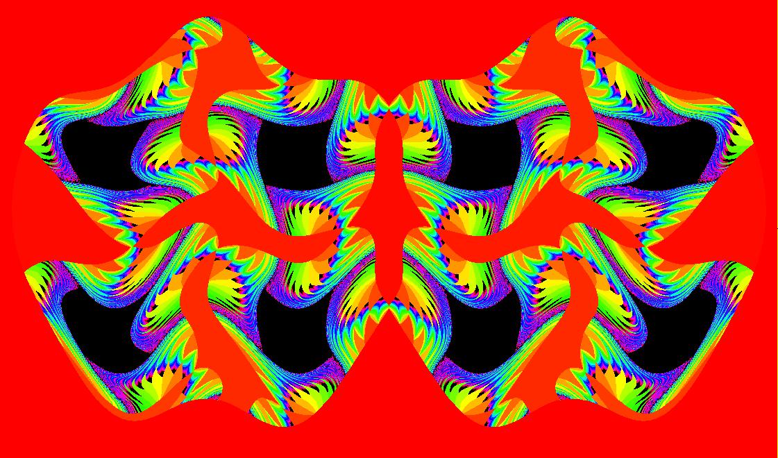
Algebraically Generated Flows Defined by Real and Complex Lines
- OdeFactory may also be used to create and edit an autonomous algebraically generated flow, an AGF for short, in R2, generated by a set of real lines of the form
L(x,y) = m*(x - c) - (y - d), λ(c,d),
and/or pairs of canonical complex conjugate lines
of the form
I(x,y) = (x - c) + i*(y - d), λ(c,d), and I, λ.
The parameters m, c and d are real numbers and λ is a complex number.
- AGFs are created by using the "Define an AGF" window shown below.
The image at the top of this document is an AGF generated by complex lines at (-1,0) and (1,0) with eigenvalues λ = +1 and -1. Moving the complex lines to (-a,-b) and (a,b) and keeping λ2 = -λ1 generates all of the Mandelbrot, fractals given by the complex quadratic iteration z <- z^2+c. Breaking the symmetry gives interesting new extensions of the Mandelbrot fractals. See the EMap view.
Section (11), Creating Galleries, walks you through two simple examples that will help you learn how to create general 1st order ode systems and AGFs using the two dialog windows.
back to TOC
(2) How to Get OdeFactory
-
OdeFactory is a Java Application program, or "App," as opposed to a Java Applet.
In contrast to a Java Applet, OdeFactory enables you to create your own systems of odes, document them, and save them to your hard drive as gallery files.
To run OdeFactory on your computer you will need:
- the Java Runtime Environment (JRE for short), which runs the OdeFactory program, and
- the OdeFactory.jar file, which contains a compressed version of the OdeFactory program.
(A) Begin by going to Verify Java Version to see if the JRE is on your computer. If it is not on your machine, you can get a free copy at the Oracle Web site.
(B) Next, download the OdeFactory.jar file to your default downloads folder, or to your desktop folder. The suffix "jar" stands for Java ARchive file. It is a compressed file like a "zip" file.
Click here to download a free copy of OdeFactory, Mac version.
Double-click the OdeFactory.jar file to open and start OdeFactory.
The first time you try to open OdeFactory.jar file on a Mac, running OS X Mavericks, or above, you will get the message:
"OdeFactory.jar" can't be opened because it is from a unidentified developer.
Select "System Preferences . . ." from the Apple menu then select "Security & Privacy" from the top row of icons. On the "General" page, click on "Open Anyway." A confirmation window opens asking if you really really really want to open "OdeFactory.jar." Click "Open."
The next time you try to open OdeFactory.jar it opens directly.
The jar file contains the entire executable program so there is no need to do any additional "install" steps.
(C) Tips regarding OdeFactory usage.
As you exit OdeFactory, the program will ask you if you would like to save any changes you may have make to any window positions and/or sizes, or to the font size in the "Ode System Comments" window. If you opt to save your changes they will be stored in a file called OdeFactoryPrefs that is created for you in the same directory as the OdeFactory.jar file. Your new window settings and font size will be used the next time you open OdeFactory.
As updates are made to OdeFactory, you can get an updated copy of the program by clicking above, or, from within the program, by selecting "Update OdeFactory" on the Help menu.
See section (15) for more detail regarding OdeFactory updates.
To delete OdeFactory from your computer, simply drag the OdeFactory.jar file, the OdeFactoryPrefs file and any gallery files you may have saved, to the trash.
OdeFactory will run from a thumb drive on any Mac that supports the JRE. Consequently you can easily carry your OdeFactory.jar, OdeFactoryPrefs and OdeFactory gallery files with you. This enables you use OdeFactory to work on differential equations wherever you have access to a Mac so you don't need to carry your computer around - in fact you don't even need to own a computer!
back to TOC
(3) The Six OdeFactory Windows
- Unlike most programs, which involve either one main window with tabs for multiple documents (for example web browsers) or several document windows (for example word processors), OdeFactory uses a main graphics window plus five dialog windows and no explicit document window. In OdeFactory you create, view, edit and manage a document, called a gallery, using functionality always readily available in the six windows together with a dozen menu items located on the Gallery and OdeSystem menus. This multi-window design, together with the small number of menu items, makes OdeFactory very easy to use since the tools you need most often are either already in view or are easy to find. An additional Help menu provides easy access to OdeFactory specific help as well as Web based help regarding Ordinary Differential Equations in general.
- The standard Windows and Mac user interfaces use slightly different designs when it comes to the placement of the menu bar and the three main window management buttons. OdeFactory uses the Windows style menu bar placement, at the top of the main window, rather than at the top of the screen, in both the Widows and Mac environments.
In the Mac environment, the standard Mac Application menu, called "OdeFactory" in this case, remains at the top of the screen. All but the "Preferences..." and "Services >" items on this menu are functional. Use the "Hide OdeFactory" item to send the entire application to the dock and the "Quit OdeFactory" item to quit the program.
- In each operating system the three window management buttons are in the standard positions. The six OdeFactory windows can be moved and resized in the usual ways. When you first open OdeFactory, default values are used for the location and size of each window. These default values may not be best for your particular screen size, however, you can customize the locations and sizes of all six windows by simply moving and resizing them. When you first exit OdeFactory, a file named OdeFactoryPrefs is created in the director containing OdeFactory. OdeFactory can save its most recent window locations and sizes in that file. OdeFactory uses your last saved values when it next opens. If you move OdeFactory to a different directory, you should also move the OdeFactoryPrefs file if you want to reuse your windows settings.
back to TOC
(4) The Main OdeFactory Window
- The main OdeFactory window is shown below on a Mac.
It contains:
- the four main menu items at the top,
- the graphics display area,
- panning arrows on the sides and corners of the graphics area,
- five view selection buttons below the graphics area,
- a coordinate and vector field display area and
- a message bar at the bottom.
The menu items are discussed starting in section (6). The graphics area, shown above for a 2D system, is the (x,y) or t = 0 plane.
Note: If you are using a two button mouse, read "clicking" to mean left-clicking. If you are using a one button mouse on a Mac, you need to use ctrl-click to simulate a right-click on a two button mouse.
- By clicking in the graphics area of the window, you can pan, start a trajectory, extend/delete a trajectory, set/check ICs, edit AGFs and select various graphic views. As you move the cursor in the graphics area, you can see the coordinate values and the magnitude of the vector field.
- To pan in the direction of the arrows, click in the border of the graphics area, near the edges, or in the corners. Panning is done in steps of tic marks. If an axis moves out of the viewing area its color changes to red to alert you to the fact that the axes no longer cross at (0,0).
- To center the view on a particular point in the graphics area, alt-click at the point of interest - or enter the coordinates of the point in the fields to the right of the Center button in the Graphics Settings dialog window, and then click the Center button.
- To center and zoom in on a particular point in the graphics area, move the cursor to the point, then, with the control key down, move the cursor away from the point in any direction. A selection square will appear. When you click the "Update" button in the "Graphics Settings" window, the view will be centered at the center of the selection square and it will be zoomed-in to the size of the square. The center and zoom feature is handy for drawing separatrices for 2D systems, locating periodic trajectories and orbits and studying the details of IMaps and EMaps (fractals).
To back out of a center/zoom just click the "Center" button in the "Graphics Settings" window. This forces a redraw which erases the selection rectangle without changing the axis parameters.
To restore the default axis parameter values after several center and zooms, set vMax = -vMin = -hMin = hMax = 5 then use the "Update" button.
- To start a trajectory at a point p = (h,v) in the graphics area, you generally just click at the point. Let "h" and "v" be the generic names of the horizontal and vertical axes respectively. The values of the axis parameters, vMax, vMin, hMin and hMax, are used to compute the values of h and v from the pixel coordinates of the cursor location. If you want to enter more exact values for h and v, R-click in the graphics area. An arrowhead is drawn on each trajectory to show the starting point and the +t direction.
For 1D systems, p = "(h,v)" = (t0,x0) and the ICs are t = t0 and x(t0) = x0. For systems of dimension greater than one, more data is needed to set the ICs. OdeFactory prompts you for additional data values as needed. To understand what additional values are needed you need to understand the primary OdeFactory views.
There are two different kinds of primary views. The first kind are projections of individual components of the solutions (called time-series) onto the viewing area. In the case of a 2D system, we have the (t,x) and (t,y) views. Call these views the "(t,a)" views.
The second kind of primary views are projections of pairs of components of the solutions (pairs of state variables) onto the viewing area. In the case of a 2D system, we have the (x,y) view. For a 3D system we have the (x,y), (x,z) and (y,z) views and for a 4D system we have the (x,y), (x,z), (x,w), (y,z), (y,w) and (z,w) views. Call these the "(a,b)" views.
Except for 1D systems, for each (a,b) primary view there is a secondary three dimensional representation of the view that you can bring up by selecting the t button in addition to two phase space buttons. These are secondary views in that you cannot define new curves in these views. Call these views the "(a,b)" views, each with its corresponding "(t,a,b)" view.
In the case of a 2D system, clicking in the graphics area at (x0,y0) sets t0 = 0 by default and sets the ICs to x(0) = x0 and y(0) = y0. (To set the default value of t0 to something other than 0, when you start the first trajectory, shift-click or shift-R-click.)
Assume a and b are phase space coordinates. Then the general rules concerning setting ICs are:
- In the (t,a) views, each trajectory can have totally different ICs.
- In the (a,b) views, when you first click on a point, t0 defaults to 0 and the location of the cursor determines initial values for a and b. If your system is not defined at t0 = 0, shift-click or shift-R-click to enter a different t0 value. Shift-click just prompts for t0, the pixel values of the cursor location are used for a0 and b0. Shift-R-click prompts for t0, a0 and b0. If additional ICs are needed, you will be prompted for them.
The additional ICs set by that first prompt are used for all subsequent trajectories defined in the (a,b) view. For example, if you have a 3D system and you select the (x,y) view, when you first click on a point in the (x,y) plane, you will be prompted for a z value. Say you set z = 1. Then in the (x,y) view you are looking along the z axis in the -z direction at projections onto the (x,y) plane of phase curves starting at (x,y,1) in R3.
In (t,a) views, you can start additional solutions with different ICs at the same (t,a) point by right-clicking in the graphics area. For example, in a 2D system you could start a solution in the (t,x) view at (t,x,y) = (1,2,3) and a second solution at (t,x,y) = (1,2,4) by right-clicking in the graphics area..
In views where both coordinates are spatial, and in the case of a 1D system, you can start multiple trajectories by dragging the cursor in the graphics area. Set dx/dt = x+y and dy/dt = y then try dragging in the (x,y) view. For a 1D example, set dx/dt = x+t, then try dragging in the (t,x) view.
When the starting point of a trajectory is a fixed point, and the horizontal axis is not t, a 1-pixel red dot surrounded by a small black circle is drawn at the starting point rather than an arrowhead. You can think of the trajectory as coming out of the screen, directly toward you. To see the solution curve as a straight line parallel to the time axis in the 3D view, click the "t" button. As you move the cursor, OdeFactory computes |v|. When |v| gets close to zero, you are often near a fixed point and OdeFactory will try to generate a fixed point solution. Consequently, fixed points can often be found by simply moving the cursor as you watch the value of |v|. Another way to find fixed points is to turn on the vector field and look for black regions. For the system: dx/dt = x+y-2, dy/dt = y-1, try moving the cursor near (1,1). Also try turning on the vector field and zooming in on black regions. For the general case, where dx/dt = f(x,y) and dy/dt = g(x,y), copying "0 = f(x,y), 0 = g(x,y)" to WolframAlpha will often produce the numerical coordinates of fixed points of the system.
In the case of 2D autonomous systems, OdeFactory can often be used to draw approximate separatrices at a saddle fixed point. First move the cursor in the phase plane and look for a likely location, where |v| is close to 0, then zoom in on the fixed point. Next move the cursor as close as possible to the fixed point. Finally, with the shift key down and the cursor located close to the fixed point, move the cursor a bit. Using this "shift-wiggle" method, trajectories can be started near fixed points even if they are not separatrices.
Approximate separatrices, and fixed points, are drawn in red and without arrowheads. Trajectories starting near or at a fixed point can be edited by clicking near the fixed point.
Since the computer screen is a pixel grid, coordinate values of the cursor position only have about three significant figures of accuracy. This is generally sufficient when you are interested primarily in the qualitative features of the solution curves. To enter more significant figures for the starting point of a solution curve, you can right-click (or ctrl-click if you have a one button mouse) anywhere in the graphics area and enter your more exact values in a pop-up dialog window. For example, if you want to set x = 1.123456 and y = 2.000459 and the closest pixel positions are x = 1.12 or x = 1.14 and y = 1.996 or y = 2.016, you can right-click or ctrl-click to enter your x and y values directly in the pop-up window shown below.
Click the tip of the arrowhead on a trajectory to:
- view a trajectory's ICs,
- extend a trajectory forward or backward in time,
- delete a trajectory, or
- check the accuracy of OdeFactory.
In the pop-up dialog window shown below, the computed values of x(t) and y(t), at the +t and -t ends of the trajectory are shown below the row of buttons. When you can find a closed form solution to the ode, these values can be used to check the accuracy of OdeFactory.
For the case shown, the example ode was dx/dt = y, dy/dt = -x with
p(0) = (0,1). The solution is:
p(t)exact = (sin(t),cos(t))
so the error in the computation at t = 100 is:
norm( p(100)exact - p(100)approx), which in WA syntax is
||{{sin(100 radians),cos(100 radians)} - {-0.506366,0.862319}}||
which evaluates to 3.809x10^-7.
- To edit an AGF, open dialog windows to edit various generator's parameters. To edit a real line's parameters, click on the line, to edit a complex line's parameters, click on the line's center. Sample pop-up dialog windows for a real line, L[1], and an imaginary line, I[1], are shown below.
You can open slider based parameter editors for AGF generators using shift-click rather than click.
- To select various graphics views of 1st order ode systems, use the five buttons labeled t, x, y, z and w below the graphics area. The t button represents the independent time variable and the other four buttons represent the dependent phase space variables.
In general, the solutions of odes are curves, defined by parametric equations, in the extended phase space R x Rn.
When two buttons are selected, you are in the "2D" editing mode. All editable views are independent of each other. For n = 2, 3 or 4, three buttons can be selected, to get to the "3D" viewing-only mode. In this mode you are seeing the "3D" view of solution curves that you have defined in the "2D" editing mode.
For a system of n 1st order odes, where n = 1, 2, 3, or 4, the number of enabled buttons is n+1 and the number of independent editable views, corresponding to the possible pairs of enabled buttons, is (n+1)*n/2. The (t,*) views are views of the component functions and the (*,*) views are 2D projections of the phase space onto the viewing screen.
If n = 1 (1D system) there is only the (t,x) view which shows the solution curves, with various ICs, in the extended phase space R x R. The phase space is just the x axis.
If n = 2 (2D system) there are four views. The three editable views are the two component views (t,x), (t,y) and the phase space view (x,y). The fourth view shows the solution curves, defined in the (x,y) view, in the extended phase space (t,x,y).
For example, the figure at the top of this document is the (x,y) view of a 2D system and the figure shown below is the corresponding "3D" (t,x,y) view of the system. The ICs for the solution curves are defined in the (x,y) view. You can not edit the solution curves in the "3D" view but you can rotate the "3D" view itself.
In the three dimensional (t,x,y) view it can become difficult to visualize the global features of a system when several trajectories are being displayed. Generally you would want to investigate a single trajectory in the (t,x,y) view, perhaps to find the approximate period of a periodic solution.
In the three dimensional (t,x,y) view, the red part of a solution curve is the +t part and the blue part is the -t part. The black trajectories in the (x,y) plane are the projections of the solution curves onto the phase space. The dots on each curve are one time unit apart.
To switch from the (x,y) view to the three dimensional (t,x,y) view, select the t button in addition to the x and y buttons. The +t axis is shown in red and is rotated a bit "out of" the screen. The x axis is shown in green, rotated a bit "into" the screen, and the y axis is shown in black in the plane of the screen. If you think of the collection of the ode's solution curves as a "body" in space, the (t,x,y) coordinate system is called the body coordinate system. The viewer's coordinate system is the "screen" coordinate system. To return to the 2D (x,y) view, deselect the t button.
When you click in the 3D viewing area the dialog window shown below opens. You can use the sliders and buttons to change the orientation of the body (ode solution curves) on the screen.
To understand how the axis rotation settings work, open the OdeFactoryExs gallery and select the first system, then select the t button in addition to the x and y buttons. You should see the extended phase space view, in 3D, of the solutions to the system "star out & star in, as an AGF," as shown above.
Click in the viewing area to open the "Set the System's Orientation in the 3D View" controller window shown above. The values of the three sliders are yaw = 30, pitch = 15 and roll = 0 as shown in the figure. You can always get back to this default orientation by clicking the "(t,x,y)" button.
Next click the "(x,y)" button to set yaw = pitch = roll = 0. This gives you the projection of the solution curves onto the (x,y) phase plane, in three space. The (red) t axis now points directly out of the screen so it cannot be seen, the (green) x axis is to your right and the (black) y axis is up. Yaw corresponds to a right hand counter clockwise (ccw) rotation of the body (solution curves), in the screen coordinate system, about the screen's vertical axis. (Note: a ccw rotation about an axis is a rotation in the direction of your fingers when your thumb points in the positive direction of the axis.) Rotate the solution curves ccw about the vertical screen-axis by dragging the yaw slider from 0 to 90 degrees. The t body-axis is now in the plane of the screen and the x body-axis is into the screen. The y body-axis remains up. So, this gets you to the "(t,y)" view in 3D and you are seeing the y(t) component of the solution curves p(t) = (x(t),y(t)).
With yaw = 90, drag the pitch slider from 0 to 90 degrees to get to the "(t,x)" view. The y body-axis now points out of the screen, the x and t body-axes are in the plane of the screen with the x body-axis pointing up and the t body-axis pointing to the right. You are now seeing the x(t) component of the solution curves.
You can also use the "(t,x)" and "(t,y)" buttons to get to the y(t) and x(t) component views directly.
To sum up, for n = 2 there are 4 views in OdeFactory:
If n = 3 or 4 we cannot view solution curves directly, since they lie in a space of dimension 4 or 5, however, we can still view components of solutions and projections of trajectories onto (a,b) as well as projections of solution curves onto (t,a,b) where a and b are any pair of phase variables.
If n = 3 (3D system) there are 10 possible views:
The case (a) views would generally be used to study initial value problems. In the case (b) views, when you select a pair of phase space coordinates, say (x,y), and start your first trajectory by clicking at (x0,y0) you will be prompted for a value for the third phase space coordinate, z in this case. If you set z to z0 then the ICs for the rest of your trajectories will have the same t0 value of 0 and the same z value of z0. When you are looking at the trajectories in the (x,y) plane, you are looking at curves in R3, starting in the z = z0 plane, that are projected onto the (x,y) plane.
The case (d) "3D" (x,y,z) view is the phase space view for a 3D system. It consists of all of the trajectories defined in the (x,y), (x,z) and (y,z) views - shown in "3D". In this view the x axis is red and out of the screen, the y axis is green and to the right while the z axis is black and up. You enter the (x,y,z) view for a 3D system by selecting the x, y and z buttons. The view opens in a default orientation. Click in the viewing area to open the "Set the System's Orientation in the 3D View" dialog window. Click the x button to exit the (x,y,z) view.
If n = 4 (4D system) there are 16 possible views:
In general, 4D systems can be very difficult to study graphically. To see a simple example of a 4D system, select "Open Examples..." on the Gallery menu and open gallery ProjectileMotion.
To sum up, OdeFactory supports 20 different independent "2D" views and 11 different dependent "3D" views.
- The message area at the bottom of the graphics window is used primarily to display the name of the current system in the current gallery but it is sometimes used to display other messages.
- The actions associated with mousing in the graphics area of the main OdeFactory window are summarized below. Assume a system has been defined.
| Mousing in the OdeFactory Graphics Area
|
| Mouse Event |
Context |
Action |
|
L-click
|
in the border
in the drawing area
on the arrowhead/seed on a trajectory/orbit
on an AGF generator
in a 3D view
|
pan in the indicated direction
start a trajectory/orbit at the cursor coords
extend/delete the traj/orbit, view details of the traj/orbit
open a text-based AGF parameter controller
open the 3D orientation controller
|
|
shift-L-click
|
in the drawing area in the Ode/IMap views
in the drawing area in the EMap view
on an AGF generator
|
if 1st click, prompt for default t0 in an (a,b) view
open an EMap color table selector
open a slider-based AGF parameter controller
|
|
alt-L-click
|
at a point p in the drawing area
in the border of the drawing area
|
center the view at p
zoom out about the center
|
|
ctrl-L-click
|
in the border of the drawing area
|
zoom in about the center
|
|
R-click
|
in the drawing area
on the arrowhead/seed on a trajectory/orbit
|
prompt for non-defaulted phase space ICs
delete the trajectory/orbit
|
|
shift-R-click
|
in the drawing area in the Ode/IMap views
in the drawing area in the EMap view
|
if 1st click, prompt for t0 in an (a,b) view
show a 4 x 4 shifted-pattern image of the EMap
|
|
alt-R-click
|
in (a,b) views, for 3D and 4D systems
|
prompt for all phase space ICs
|
|
move
|
in the drawing area
|
show the cursor coordinates
|
|
ctrl-move
|
in the drawing area
|
open a "center & zoom" rectangle then click "Update"
|
|
drag
|
in the drawing area
on a complex generator
|
start multiple trajectories/orbits
change the vector field
|
|
shift-drag
|
near a saddle point of a 2D system
|
draw approximate separatrices
|
|
shift&ctrl-L-click, shift&alt-L-click
|
select UL corner of cropping rect then select LR corner of cropping rect
|
crop image using a rectangle
|
The other five OdeFactory windows are supporting dialog windows. They are discussed in detail in section (10) of this document. However, before reading about those windows it is best to familiarize yourself with the Gallery concept and the OdeFactory menus.
back to TOC
(5) The Gallery Concept
- Early applications programs were often thought of as being used to create and edit a single "document" such as: a text document, a spread sheet, a drawing, a data base document etc. Generally the user could have several documents open at the same time, and could copy/paste between documents, but each document was stored in its own file.
- Later, as more complex applications were needed to create, edit and manage collections of items, that could themselves be thought of as documents, such as: emails (Mail), photos (iPhoto), songs (iTunes), web pages (Firefox), Java classes (BlueJ) etc., the notion of a "document" had to be expanded. Applications evolved into development environments. The primary "document" being worked on generally organized and managed several more basic secondary documents that could be collected and/or edited.
- OdeFactory is a development environment for studying systems of odes. In OdeFactory, a gallery is a named collection, of named systems of odes, that can be saved to the hard drive. A gallery is the primary "document" being viewed and/or worked on. When using OdeFactory you are always working within the context of a gallery. Opening an existing gallery enables you to work with a copy of the gallery, which we call in general the "working gallery." If you don't open a gallery, the working gallery is just the default (initially empty) gallery called "untitled." You should note that OdeFactory only allows you to work with a single working gallery at a time.
- When you open a gallery and then select and open a system of odes from the gallery you are creating a working copy of: the system of odes plus the viewing environment for the system of odes, which we will call the "working system." You can think of the working system as a secondary document.
- To study the working system you can make changes to the viewing environment such as: adding/editing trajectories, adding views, changing graphics settings and/or editing the system's comments. If you want to save any changes you may have made to the working system, in the working gallery, you must update the system in the working gallery before you switch to a different working system. You can switch to a different working system either by editing the working system equations, by selecting a different system in the working gallery, or by selecting "Define New System" from the OdeSystem menu. If you switch to a different working system, you can add the new ode system to the working gallery by selecting "Add to Gallery" from the OdeSystem menu. Finally, if you want to save all of the changes that you made to the working gallery, you must select "Save As" from the Gallery menu before you open a different gallery, or, answer "yes" when asked if you want to save the current version of the working gallery as you exit the program.
back to TOC
(6) The Gallery Menu
- OdeFactory enables the user to: view, create, modify and save galleries via the Gallery menu. Menu items with the icon
 give you easy access to internet-based ode resources. They appear on the various menus if you open an internet connection before you enter OdeFactory.
A permanent copy of a gallery may exist on the Web and/or locally on your computer's hard drive. When you are in OdeFactory you are using a "working" copy of a gallery.
On the Gallery menu, select:
- New... to create a new working gallery of ode systems on your computer. When asked to name the new gallery, you may use whatever name you care to. No extension is required on OdeFactory gallery names, however, you may add one if you want to make it easier to identify OdeFactory gallery files in your list of files. Note that when you first enter OdeFactory, a default gallery called "untitled" is created so you only really need to use New... if you need to exit from the current gallery before you begin creating a new gallery. When the working gallery is the default gallery, you can effectively create a new gallery by simply saving the default gallery with a new name.
- ------------------------------
- Open Local... to select and open a gallery residing on your computer.
- Open URL... to enter a URL and open a gallery residing on the Web.
- Open Examples... to select an example gallery from the OdeFactory.com Web site.
Currently the 38 sample galleries on the selection list contain about 1900 sample systems with about 2800 images. Opening a sample gallery in OdeFactory and experimenting with the various systems is a good way to learn how to use the program while at the same time studying dynamical systems. You can also save a copy of any sample gallery to your computer and then create your own custom version of the gallery.
Click on the hypertext links in the following list to see a slide show of the galleries contents. If you download a copy of OdeFactory, you can open any sample gallery on the list and experiment with the various systems yourself. The "Save as Html" item on the OdeSystem menu was used to create the slide shows.
Each slide show has a grid of thumbnail images at the top. The thumbnails act as a table of contents for the systems in the selected gallery. Click on a thumbnail to scroll to the system associated with the image.
****** 13 General OdeFactory Galleries ******
- OdeFactoryExs - 79 systems used to demonstrate OdeFactory features
- VectorFields - 137 systems showing how to build vector fields
- ShortDemos - 96 systems that demonstrate some advanced OdeFactory features
- DynamicalSysExs - 45 examples of real-time animation using OdeFactory
- 1DSystemExs - 15 sample 1D and 2D Ode systems
- IterationExs - 15 examples of Newton's method and Euler's method
- 2DLinearVectorFields - 31 examples used to classify 2D linear Odes and IMaps
- 3DViewExs - 5 systems that demonstrate how to use 3D views
- SeparatrixExs - 33 examples that demonstrate how to draw separatrices
- PeriodicIMapOrbits - 60 examples showing how to find periodic orbits in IMaps
- PhysicsExs - 57 examples of Physics applications
- Sprott'sChaoticFlows - 19 simple chaotic systems from Prof Sprott
- Connections - 85 examples illustrating connections between various concepts
****** 9 Textbook/Test Galleries ******
- StrogatzExs - 39 examples from Prof Strogatz's book
- Hubbard&WestPartI - 19 examples from Hubbard & West, "Differential Equations"
- PerkoExs - 33 2D and 3D systems from Perko's DE and Dynamical Systems book
- B&DiP - 24 examples from Boyce and DiPrima's classic ode text, edition 8
- DELW - 18 "Differential Equations Lab Workbook" examples, see Help menu
- Classic - 25 classic systems discussed in many introductory ode textbooks
- PaulsExamples - 17 examples from Paul's on-line Math Notes
- SOSExamples - 9 examples from the on-line course S.O.S. Mathematics Odes
- PlottingCurves - 90 systems showing how to use OdeFactory to plot curves
****** 16 IMap/EMap/Fractal Galleries ******
- MapExs - 113 examples (images only) showing how to view 1D and 2D ode systems as IMaps/EMaps
- EMapExs - 27 examples showing how to view 2D ode systems as Julia sets (fractals)
- IMapSeparatrixExs - 19 examples showing how to find IMap separatrix systems
- ArtGallery - 162 examples of "Interactive Art" using IMaps and EMaps
- HopalongEMaps - 90 examples (images only) of EMaps based on a variation of the hopalong map
- FamilyOfEMaps - 34 examples that show how to create variations of EMaps
- InfiniteImages - 108 abstract "Art" (images only) created from a single system
- Patterns - 126 abstract "Art" (images only) created from a single system
- VacationArt - 180 abstract "Art" (images only) created from related systems
- ClassicFractals - 62 Mandelbrot and Julia set examples, Sierpinski gasket, Barnsley Fern
- PowerFractals - 60 examples of Julia sets/bifurcation diagrams using: z<-z^n+c, n=2...6
- FractalCenters - 15 examples of localized fractals
- AGFEMapExs - 18 examples of Julia sets related to AGFs
- AGFEMapExsB - 28 more examples of AGFs and EMaps
- AGFractals - 21 examples of Julia sets generated directly from AGFs
- AGFs&Mandelbrot - 20 examples showing how to write z<-z^2+c as an AGF
- ------------------------------
- Save As... to save, or reSave, a copy of the working gallery. The working gallery file will be saved to your hard drive and the full file name of the gallery file will be saved in your OdeFactoryPrefs file.
Save As... does not change the name of the working gallery. For example, if your working gallery is named "untitled" and you save a copy as "MyNewGallery," the working system will still be called "untitled" since the name of the working gallery did not change. However, if you next use "Open Local" and select "MyNewGallery" the system selection list title will change to "Systems in: MyNewGallery" since "MyNewGallery" is then the name of the working gallery.
Note that any working gallery can be saved to your hard drive. Consequently once you open a gallery on the Web, you can save a copy of that gallery to your hard drive.
If you have saved any galleries during your OdeFactory session, your last saved gallery, presumably the one you were working on, will open automatically the next time you enter OdeFactory.
- ------------------------------
- Show All Comments to create a window containing all of the comments associated with the ode systems in the working gallery. The window opens on top of the system comments window. You can drag it to a different location and resize it as needed.
One purpose of the window is to provide you with a view of a gallery's contents, without having to open each system in the gallery. If you copy/paste all of the comments into a text processor, you can spell-check them, find key words and/or print the comments. Note that if you change a comment for a system in the current gallery, or switch to a different gallery, while the Gallery Comments window is open, its contents will no longer be up-to-date. To up-date the contents use the "Refresh Gallery Comments" button at the bottom of the Gallery Comments window or close/reopen the window. Red text is used at the top of the window to serve as a reminder that the contents is context sensitive.
The Gallery Comments window can be also be used to add an overview to a gallery. The trick to doing this is create a first system called " Overview" and enter the system's comments as the overview of the gallery. The space at the start of the name forces it to the top of the list of systems.
There is a second button at the bottom of the Gallery Comments window that enables you to toggle the size and font between Presentation and Computer Screen size.
To change the size of the font in the window, place the cursor in the window and use ↑/↓ to increase/decrease the size of the font.
back to TOC
(7) The OdeSystem Menu
- OdeFactory enables the user to manage ode systems in a gallery using the OdeSystem menu. In OdeFactory, the term "ode system" refers to the equations defining the system plus the "viewing" environment. The viewing environment consists of various user defined views of trajectories and comments regarding the system. The equations are the most significant part of the definition of an "ode system" in OdeFactory so if you change a parameter value you are changing to a new system.
- On the OdeSystem menu, select:
back to TOC
(8) The Settings Menu
- These next nine menu items are options that can be toggled on/off during an OdeFactory session. The default state for each option is off.
On the Settings menu, select:
- Show ToolTips to turn the tool tips feature on.
- ------------------------------
- Show Colored Vector Field w/Nullclines to enable the colored 2D vector field with nullclines feature.
To locate a fixed point of a 2D system of odes, center on an intersection of the yellow nullclines and zoom in. The small black region contains a fixed point. If the fixed point is a saddle, starting two trajectories near opposite edges of the black region generally produces the separatrix system associated with the fixed point.
- Show EMap w/Max Detail to generate a more detailed version of an EMap image.
- Set the EMap Prison Shape to Square to toggle between the classic circular prison of radius sqrt(50) centered at the origin to a 14X14 square prison centered at the origin in the EMap or EMapMax view.
- Show EMap Images in HD to render EMap images in HD. NOTE: this item does not appear on the Help menu if you are not using a Mac with a Retina display.
- Show Last +t Point to display the location of the last point on the last trajectory that was started. The coordinates appear in the message field below the graphics area with full 16 digit precision.
- Hide 2D Ode Trajectories to replace the arrowheads with dots and hide the trajectories in the Ode view of 2D systems.
- ------------------------------
- Show 2D IMap Orbit Sequence to enable the drawing of line segments in the (x,y) plane between successive iteration points for a 2D IMap iteration sequence.
- Show Approximate Period to compute an estimate of the period of the last 2D Ode trajectory, or 1D or 2D IMap orbit, that was started. As a side effect, the total number of orbits in the case of an IMap is also given. The estimate of the period appears in the message field below the graphics area.
- Hide Axes to hide the display of the coordinate axes.
- Hide Arrowheads/Seeds to hide the display of arrowheads/seeds on trajectories/orbits in the Ode/IMap views of 2D systems.
back to TOC
(9) The Help Menu
- The Help menu provides help using OdeFactory as well as Web access to general information regarding the theory of odes.
On the Help menu, select:
back to TOC
(10) The Five Dialog Windows
- To make it easy to define and study systems of odes and manage systems in galleries, five supporting dialog windows automatically open near the main window when OdeFactory starts up. All of the windows will fit on your screen if you have a resolution of 1440 x 900 pixels or more. The first time you open OdeFactory each dialog window opens at a default location and with a default size. All six OdeFactory windows can be moved and resized and the locations and sizes can be saved in the file OdeFactoryPrefs as you exit OdeFactory. The dialog windows enable you to:
- view/edit comments for a particular system of odes,
- select particular systems for study from a gallery,
- define a general first order system of odes,
- define AGF systems of odes and
- modify the graphics settings
The various dialog windows communicate with the program via text fields and context sensitive buttons. The names on the buttons are short-hand for commands. For example, when you click the "Z In" button you are asking OdeFactory to zoom in on whatever is in the viewing area. When you click the "V On" button you are asking OdeFactory to display the vector field. The action of a button and the text on a button will change, or the button may become disabled, when a change of context renders the command meaningless, or inappropriate. For example, if you switch from a 2D system to a 1D system, the "V On" button changes to the "S On" button since it would then be appropriate to view the slope field in the (t,x) plane, but not appropriate to view the vector field on the x axis. If you switch to a 3D or 4D system, the "V On," or "S On," button is disabled.
The five dialog windows are:
- The Ode System/Gallery Comments window. - This dual purpose window is used to view/edit a selected system's comments or to view all of the comments associated with all of the systems in a gallery.
Use ↑/↓ to increase/decrease the size of the font in this window. Your current font size can be saved in the file OdeFactoryPrefs as you exit OdeFactory.
A default system comment, consisting of the equations, parameters and any user defined functions, can easily be created by using the Insert Equations button. Whenever you edit an ode system's comments, you must use the Update in Gallery item on the OdeSystem menu to save your changes.
The "View Gal Cmnts/Edit Sys Cmnts" button is used to toggle between viewing all of the comments associated with the systems in a gallery and viewing/editing the comments for the currently selected system in the gallery. When the button label is "View Gal Cmnts," clicking the button means you want to view the gallery comments. When the button label is "Edit Sys Cmnts," clicking the button means you want to edit the currently selected system's comments.
As you enter the "view gallery comments" mode OdeFactory generates a list of all of the current comments for all of the systems in the gallery. The text color switches to red to remind you that you can't edit text in this mode. In this mode you get an overview of a gallery's contents, without having to open each system in the gallery. If you copy/paste all of the gallery comments into a text processor, you can spell-check the comments, find key words and/or print the comments. If you change a system's comments, the changes will be made in the gallery comments.
If you want to connect your computer to a projector system and give a lecture or a presentation while using OdeFactory, use the "Presentation Size/Computer Size" button to toggle between a large (projector) size of the Ode System/Gallery Comments window and a computer-screen size of the window.
- The Systems in: current gallery window. - This window displays an alphabetized selection list of the systems of odes in the currently open gallery. Click on a system name to select and open the ode system. You can also Rename ode systems in a gallery and Delete ode systems from a gallery using the buttons at the bottom of the window - however, these changes to the gallery will not become permanent until you use "Save As..." on the Gallery menu to re-save the gallery.
- The Define a General 1st Order Ode System window. - This window enables you to define a general first order system of odes by entering the right hand sides of the system or by entering the ode in the normal form, i.e. the "y(x) form." You may also enter any parameters and user defined functions that you may need. Changes entered in this window do not take effect until you click the "Update Eqns, Params &/or Fns" button.
When the params field is not empty, you can use the "Adj Ctrl Params..." button to open a ode system specific dialog window containing a list of scaled sliders, one for each parameter in your system. You can watch the effect various parameter values have on solution curves, vector fields, IMaps, PMaps and EMaps by adjusting the sliders slowly, using the +/- buttons, or rapidly by dragging a slider or by clicking in a slider's range bar.
If the view of your system contains a lot of trajectories you may need to change parameter values slowly since all of the trajectories need to be recomputed as parameter values change. If you are viewing a EMap (fractal), wait for the redraw before going to a new parameter value.
Since each parameter controller is system-specific, OdeFactory prohibits you from changing to a different system while the current system's parameter controller window is open. The red text is used to remind you to close the window before you switch to a different system.
The real-time parameter controller is useful when you are looking for bifurcation values for systems of odes or when you are studying iteration maps or Julia sets. Select "Open Examples..." on the Gallery menu to access the sample gallery "StrogatzExs" if you want to experiment with adjusting control parameters. See the figure shown below.
Note: since the slider scales are limited to 100 selection values in either direction, you can only adjust parameters to two digits of precision using the sliders. If you want more digits of precision you can enter parameter values directly into the "params:" field of the "Define a General 1st Order Ode System" window then hit the "Update Eqns, Params, Fns" button.
The range limits on the sliders are [-10n,10n] for n = -1, 0, 1, 2, 3. They can be changed by factors of 10 as follows. To increase the range interval for a parameter by a factor of 10, place the slider at either end of the range scale and click the "Adj Ctrl Params..." button again. To decrease the range interval by a factor of 10, place the slider between -10 and +10 on the scale and click the "Adj Ctrl Params..." button again. The newer versions of the parameter controller open on top of the older versions. You can move them off of each other and close any you no longer want to use, or for some systems, it may be convenient to leave more than one controller open so you can use different controllers for different parameter ranges.
Any change to the parameter values creates a new version of the working ode system which will not be in the working gallery until you select the "Add to Gallery" item on the OdeSystem menu. To study the effect of using different values for a parameter in an ode, it is sometimes convenient to create a family of related versions of a system. An example would be: "(y,-x+a*y), a = .00", "(y,-x+a*y), a = 1.00" and "(y,-x+a*y), a = 2.00" where the system names are just the default named generated by OdeFactory.
Syntax rules for the text fields in this window follow.
- The right hand sides of the differential equations may contain:
- integer and floating point numbers
- reserved variable names: x, y, z, w and t
- constant names: e and pi
- the arithmetic operators: +, -, *, /, and ^
- standard functions names: abs, sqrt, sin, cos, tan, asin, acos, atan, ln, log, sinh, cosh, tanh, exp, step, sgn and max and min
- user defined parameter names (single lower case letters other than x, y, z, w, t, e, i, j, l, o, u and v)
- user defined function names (single upper case letters)
- right and left parens and commas in the min and max functions
- you can not leave gaps in the list of right hand sides, for example, if there is an expression defining dz/dt, there must also be expressions defining dx/dt and dy/dt
- A user defined parameter list:
- has the form: name = val; name = val; ... name = val
- a sample parameter list is: a = -1; b = 2.5
- semicolons are used as a delimiters in the list
- A user defined function list:
- has the form: name = expr; name = expr; ... name = expr
- a sample user defined function list is: P = x-sin(x+y); Q = a*x^2-b*y
- semicolons are used as a delimiters in the list
Note: the right hand sides of user defined functions may contain user defined parameters but not user defined functions. Processing the right hand sides of the differential equations involves two scans of the user input. The first scan replaces the user defined function names with the expressions that define the functions and the second scan replaces the user defined parameter names with the numeric values of the parameters.
- A user defined ode of degree 1 through 4 in the "y(x) form:"
- is entered as: y' = F(x,y) or y'' = F(x,y,y') or ... y'''' = F(x,y,y',y'',y''')
- for example: y''' = a*sin(x) + 2*x + y - P*y''^2
- the use of constants, such as a is OK
- the use of functions, such as P, is also OK but functions must be defined in terms of variables (t,x,y,z,w), not (x,y,y',y'',y''')
- The Define an AGF window. - This window enables you to define AGFs by adding specific real linear generators and canonical complex linear generators to the flow. To add a vertical real line, use "inf" for the slope of the line.
To edit and/or delete an existing real line, click on the line and then edit its parameters in the pop-up dialog window.
Complex linear generators are added in conjugate pairs and have the general form: I = a*(x-c)+b*(y-d), λ, where a, b and λ are complex numbers. The canonical complex linear generators have a = 1, b = i and re(λ) and im(λ) equal to -1, 0 or 1. In general, the second component of the eigenvector belonging to λ is -a and the first component is b.
To edit and/or delete a complex line, click on the line's green center then edit its parameters in the pop-up dialog window.
Additions or deletions of real or complex generators, or changes to parameter values of existing generators, creates a new working ode system which will not be in the working gallery until you select the "Add to Gallery" item on the OdeSystem menu.
- The Graphics Settings window. - This window, shown below, is used to modify the view of the solutions of the ode being studied. In the dialog window:
- Edit hMin, hMax, vMin and/or vMax to change the horizontal and/or vertical viewing area parameters. The tab order for these buttons is: hMin -> hMax -> vMax -> vMin. When the origin is within the viewing area, both axes cross at the origin and are drawn in black. When the origin is outside of the viewing area one or both axes through the origin would be outside of the viewing area. axes that would be outside of the viewing area are shifted back into the viewing area and are drawn in red to alert you to the fact that the crossing point is no longer (0,0).
Note: any changes you make in the hMin, hMax, vMin and/or vMax fields for the viewing area will not take effect until you click the "Update" button.
- Click the Z In/Z Out button to zoom in/out about the center of the viewing area.
The radio buttons to the right of the zoom button toggle the Z In/Z Out states. The zoom range is on the order of 106 to 10-6, in system coordinates.
An alternate way to zoom-in is to ctrl-L-click in the border of the drawing area. Doing an alt-L-click in the border will cause a zoom-out.
- Click the Center button to center the viewing area at the system coordinates shown in the two fields to the right of the Center button - or, simply alt-click in the graphics area at the point you want to center on.
You can also use the center button to simply refresh the graphics.
Note: the hMin, hMax, vMin, vMax fields, and the two center-of-the-view coordinate fields to the right of the Center button, are synchronized input/output fields. As you pan, the values in all six fields will be updated. If you edit any of the hMin, hMax, vMin or vMax values, and then hit the "Update" button, the two center-of-the-view coordinate fields will be updated. If you edit the values in the two center-of-the-view coordinate fields then hit the "Center" button, the hMin, hMax, vMin and vMax values will be updated. Zooming is about the center-of-the-view so zooming will change the hMin, hMax, vMin and vMax values, but not the center-of-the-view coordinate values.
- Click the Flow button to create an animation of the flow.
A flow animation consists of red dots moving forward in time or blue dots moving backward in time in the phase space. A dot starts at the arrowhead on each trajectory, by default, and additional dots can be started at random locations in the graphics area. The dots move in the phase space under the action of the vector field.
When you click the Flow button, the pop-up dialog window shown below opens which enables you to adjust the number of the random dots from 0 to 150, the speed of the dots from Min to Max, the duration of the animation from 0 to 180 seconds and the direction of the flow of the dots in time.
The speed of the dots, which is proportional to |v| at each dot's location, can vary over the viewing area by an order of magnitude. The "Speed of dots" slider enables you to slow down the dots to get a better overview of the flow's dynamics. The dots are slowed by introducing a delay between each redrawing of the dots. The Min speed corresponds to a 200 millisecond delay and the Max speed corresponds to no delay.
You can move the sliders on the slide bars by dragging them or by simply clicking at various positions on the slide bars.
A dot that leaves the viewing area will reappear if the dot's trajectory reenters the viewing area.
Each time you click the "Start Flow" button, a new animation is started. For example, if the number of dots is 20 and the duration is 10 seconds, when you click the "Start Flow" button three times in quick succession, say one second apart, you will see 20 dots created on your first click, 20 more dots created on your second click and 20 more dots created on your third click. The three animations will run concurrently, each for 10 seconds, and they will end one second apart.
While an animation is running you cannot change the system of odes or the view of the solution curves. The message bar below the graphics area shows the time left in the animation.
If you want to clear the animation dots from the graphics area after an animation stops, you can force a redraw of the graphics area by hitting the "Center" button.
For another animation of flows defined by vector fields, see the applets 2-D Vector Fields and 3-D Vector Fields by Paul Falstad.
- With coloring turned on in the Help menu, click the V On/Off button to turn a scaled view of the colored vector field on/off for 2D autonomous systems. Arrows point in the direction of the vector field. The length of each arrow is scaled so that the arrows do not overlap in the display area. The relative speed of the flow is indicated by the length of each arrow. Regions with the same color indicate the same speed. The black end of the color chart indicates |v| is small, the pink end indicates |v| is large. Fixed points can be located by looking for black regions and then zooming in on them. In the image below, there is a fixed point at the origin.
When a 2D system has parameters, OdeFactory considers the system autonomous only if it is autonomous for all values of the parameters. When a 2D system is nonautonomous, the V On/Off button is disabled since the vector field is time dependent and each point in the phase space would need to show multiple vectors.
If you want to watch the vectors change continuously as you move a parameter slider, be sure to first turn coloring Off on the Help menu. If you want to make a large change in a parameter value, you can leave coloring On and simply click in the slider bar - but be sure to wait for the redraw before clicking again!
Note: if you want to see the true magnitude of a particular arrow shown in the scaled vector field, place the tip of the cursor at the back end of the arrow and view the coordinate display at the bottom right of the graphics area. The true value of the vector field is of course used in the computation of all solution curves.
- Click the S On/Off button to turn a view of the slope field on/off for 1D systems.
Note: the S On/Off and V On/Off "buttons" are a single context dependent button in the Graphic Settings window. The label on the button and the functionality of the button depends on the system under consideration.
- Click the Bdr button to stop solutions at the border of the viewing rectangle. When the border is red, the button turns green. Clicking it when it is green means turn the border green and allow solutions to cross the border.
You would want to stop a solution at the border if the ode is not defined at the border. For example, dx/dt = x*t/((x+2)*(t-3)) is not defined at x = -2 and at t = 3 so RK4 will fail if a solution attempts to cross these lines. To plot the solutions, begin with the default viewing area (vMin = hMin = -5, vMax = hMax = 5) and start some solution curves. You will get jaggies as RK4 fails at x = -2 and t = 3. Pan up until vMin = -2 and left until hMax = 3 then click the Bdr button. The jaggies at the border will vanish.
- Click the Clear button to clear all solution curves in the viewing area. The equations themselves are not cleared.
- Click the R2/R2+ button to toggle between the R2 and R2+ views of a
2D flow.
Note: The R2+ view, called the Poincaré compactification of R2, is used to study critical points at infinity for 2D Ode systems. It is generated as follows: (1) place the origin of the xy plane at the north pole of the unit sphere, (2) project the flow from the xy plane onto the top half of the sphere's surface through the center of the sphere, (3) project the flow on the sphere's surface perpendicularly down onto the plane containing the sphere's equator. R2 gets mapped to the unit disk, R2+. All points in R2 outside of the unit disk get mapped to the edge of the disk in R2+. Coordinates (u,v) are used in the R2+ view, where
u = x/sqrt(1+x^2+y^2)
v = y/sqrt(1+x^2+y^2),
rather than (x,y). The R2+ view of a flow is used to display the global phase portrait of the flow.
The figure shown below, from my book on
AGFs, page 17, illustrates the Poincaré compactification mapping. In the book I used E2 and E2+ instead of R2 and R2+ which are used in OdeFactory.
For more details, look for "Poincare's sphere" in
Perko's book, "Differential Equations and Dynamical Systems," second edition.
The OdeFactory R2+ view of the system shown in Figure 1.1 above is shown below.
- Click the Ode/IMap/EMap button to toggle between the Ode, IMap and EMap views.
For 3D and 4D systems, only the Ode view is available. For 1D systems, both the Ode and IMap views are available and for 2D systems all three views are available.
The default view, which is used whenever you create a new system or open an existing system, is the Ode view. The text on the Ode/IMap/EMap is the name of the next viewing state, that is, the state you will be in if you click the button. So - if you are in the Ode state, the button text is IMap. As a reminder of your current viewing state, the message in the message bar below the graphics area starts with the name of your current viewing state.
The three different views are the result of applying different iteration algorithms to the mapping defined by the vector field and applying different display algorithms to the results of the iterations.
For a discussion of how to create interesting IMaps and EMaps, see: Q&A 44.
In the Ode view, the iteration algorithm is the RK4 numerical method which is commonly used to "solve" systems of odes. Each iteration involves four evaluations of the vector field near the current point. The new point is .01 time units from the old point. Each trajectory, or solution curve, consists of 20,000 very short line segments connecting the iteration points, 10,000 in the +t direction and 10,000 in the -t direction. The shortness of the line segments makes the solution curves look continuous and smooth. The start of the iteration is specified by the ICs for the ode and the corresponding starting point on the trajectory is indicated by an arrowhead. For an 2D system, drawing one solution curves requires 80k evaluations of the vector field.
In the IMap view, the iteration algorithm itself is much simpler (only one evaluation of the vector field at each point instead of four) and the iteration steps are effectively 100 times longer. The new point is one step (which you might think of as one "time" unit) from the old point. The "trajectory," now called an orbit, is drawn as a set of straight line segments between the iteration points for 1D systems and as a set of unconnected dots for a 2D system, in the 2D view. If you view a 2D IMap in the 3D/(x,y) subview, you will see straight line segments connecting the iteration points. Each orbit is drawn in the +t direction only and it consist of 100 steps. The starting points for orbits are called "seed" values. To draw an IMap, start several trajectories in the Ode view, then toggle to the IMap view. The seed points look the same in the IMap view as the other points on an orbit. They correspond to the arrowheads in the Ode view. You can also start orbits directly in the IMap view by clicking or dragging in the graphics viewing area while in the IMap view. In the IMap view, each orbit is colored with one of 5 different colors: black, blue, ref, green and magenta. If there are more than 5 orbits, the colors are recycled.
If you start several orbits in the IMap view, you will need to force a redraw to see the different colors of the orbits. An easy way to force a redraw is to click the "Center" button in the "Graphics Settings" window. In the 3D view, the (t,x) and (t,y) subviews are step series views of the iterations.
For a 1D system, an IMap iteration is, for n = 0, 1, 2, . . .
xn+1 ← f(tn,xn),
tn+1 ← n.
The initial point, (0,x0), is called the "seed" value and the successive values of x are shown in the (t,x) plane as a time series connected by straight line segments.
For a 2D system, the IMap iteration is, for n = 0, 1, 2, . . .
xn+1 ← f(tn,xn,yn),
yn+1 ← g(tn,xn,yn).
tn+1 ← n.
The initial point, (0,x0,y0), is called the "seed" value. The successive values of (x,y) are shown as small (1-pixel) colored dots in the phase space and as dots connected by line segments in the extended phase space, i.e. in the 3D view. The 3D/(t,x) and 3D/(t,y) views show the time series components of the iteration.
Most common iteration maps are autonomous systems, that is, they have no explicit dependence on tn, that is, the iteration index n. Nonautonomous IMaps are possible in OdeFactory, they just correspond to nonautonomous vector fields.
A vector field defining an interesting ode will generally not produce an interesting iteration map and visa versa. For some interesting IMap examples, select "MapExs" from the Gallery/Open Examples menu. Select a system and toggle the button between the Ode, IMap and EMap views of the system.
Aside: for 2D driven systems, when the driving functions are just sin(. . .t. . .) and/or cos(. . .t. . .), in addition to the iterative map, a Poincaré map (which I call a PMap) is also available. To see the Poincaré map, see the 3D/(x,y) view.
The following is an example of the 2D view of an IMap that uses 31 seed values. The system is defined by the iteration:
x <- y-abs(x)/x*sqrt(abs(b*x-c)),
y <- a-x%d
with parameter values of
a = .54; b = .43; c = .84; d = 69.00.
The sgn(x) function could be used in place of abs(x)/x.
You can Zoom In/Out, change the parameter values and view the IMap in R2+ as well as in R2. The Ode view of the system is less interesting than the IMap view. See sample gallery MapExs for other interesting IMaps defined by 2D systems of odes.
Six orbits starting at (0,.5), (.5,1), . . . (2.5,3) for the 2D IMap (y,-x) are shown below in the 3D/(x,y) view.
In the EMap view, the same simple iteration algorithm is used as in the IMap view but the display algorithm is entirely different from the display algorithms used in the Ode and IMap views.
You can use the EMap view in OdeFactory to study fractals. For complex maps of the form z <- R(z) = P(z)/Q(z), where P and Q are polynomials in the complex number z = x+i*y, the EMap view shows the Julia set associated with the 2D vector field.
The EMap is constructed using the escape time algorithm as follows:
- create a table of K colors indexed by iteration step k
note: one iteration step is being thought of as one "time" step
- set a bailout value M (used to terminate a potentially infinite iteration)
then . . .
- for each pixel in the graphics area (x0,y0), written in screen coordinates, and starting with k = 1, iterate until xk2+yk2 > M or k > K
- if the iteration ends with xk2+yk2 > M, use color k (the color coded "escape time") to color the starting point, (x0,y0), else use black (to indicate no escape)
Note 1: the test for an escape is NOT applied to the seed point itself, (x0,y0), but to the first iterate of the seed point - however it is the seed point that gets colored.
Note 2: it is the first "escape" that counts. A point could possibly escape, on iteration 5 say, then return for the rest of the iterations - but that still counts as an escape.
A simpler statement of the EMap algorithm, as implemented in OdeFactory, is:
- set bailout value M = 50 and color table size K = 100, then
- for each pixel in the viewing area, define a seed point, set k = 0 and
- iterate until either:
- (a) the first iterate of the seed point leaves a circle of radius sqrt(50) = 7.07 centered at the origin or
- (b) the iteration step k is greater than 100, i.e. the size of the color table.
- if (a) terminated the iteration the seed point "escaped," color the point color k else (b) the seed point did not escape, color the point black.
- NOTE: there is an EMapMax option on the Settings menu that increases K to 512. It produces a more detailed version of the prisoner set. It should be used when searching for the separatrix system of an IMap.
Here are a few things to note about EMap images:
- the escape time algorithm is more of a display or viewing algorithm than a "Mathematical" algorithm
- EMaps for smooth systems are often floral fractals, for nonsmooth systems they are generally geometric and most often they are not fractals
- EMaps depend strongly on the particular system parameter values AND on the viewing parameter values: dimensions of the viewing area, M, K and the color table
- the "same" system can generate an essentially infinite number of EMap images
- you can't reproduce an EMap image without knowing the exact system and the exact viewing parameter values
- relatively small values of M and K are used to speed up the algorithm
- the "escape time" is a color encoding of iteration steps
- an iteration step is thought of as 1 unit of "time"
- black regions are called "prisoner" sets (no escape within K steps)
- "time" can be modified by multiplying the vector field by a parameterized scale factor such as (1+s*0.1)
For the Mandelbrot quadratic iteration, z <- z2+c, once a point "escapes" it escapes to infinity so using a bailout value in the algorithm works for finding the Julia sets. For more general iteration maps, a point may escape from a circle of radius sqrt(M) and return to points within the circle for later iterations. Consequently, calling the EMap view the JSet view would not be correct in general since the escape time algorithm does not produce Julia sets for all iteration maps.
The escape time algorithm does not use the list of starting points that define the ICs/seeds for the trajectories/orbits in the Ode and IMap views. Instead it starts a temporary test orbit at each pixel in the graphics area and the escape time of the test orbit is used to assign a color to the pixel in the EMap image.
The escape time algorithm can be used on all 2D vector fields but not all 2D vector fields produce interesting images. A well known class of 2D vector fields that do produce interesting images, which are actually fractals, is defined by the iteration z <- zn+c where z = x+i*y, c = p+i*q and n is an integer great than 1.
For a 2D EMap, coloring one pixel requires from 1 to 100 evaluations of the vector field. The graphics area in the figure shown below contains about 300k pixels so drawing the EMap requires from 300k to 30000k evaluations of the vector field. The 100 evaluations worst-case corresponds to an entirely black EMap. Before OdeFactory draws a EMap, 1000 random points in the graphics area are sampled and if more than 99% of them are black the graphics area is simply colored black. This reduces the drawing time by a factor of 300 for uninteresting EMaps. For interesting EMaps, the average number of iterations per pixel is generally much less than 100 and the drawing time is on the order of a few seconds. When parameters are involved, if, while the image is being generated, it looks like the image will not be interesting, changing a parameter value before the drawing completes will abort the drawing and start a new drawing using the new parameter value.
The EMap view can require much more time to complete than an Ode or IMap view since an iteration is started at each pixel in the graphics area. You may do a zoom, pan, recenter or parameter change while a EMap is drawing but you are prohibited from changing the view to the Ode or IMap view.
Shown below is a EMap view for the system,
z <- z^2+c
where z and c are complex numbers. In OdeFactory, the system is entered as the vector field
v = (x^2-y^2+p,2*x*y+q)
where
p = -.7321 and q = .2165.
The viewing area is from hMin = -.88 to hMax = -.68 and from vMin = .05 to vMax = .5. Get into OdeFactory and open sample gallery "EMapExs" and select system "c = -.7321+.2165*i" if you want to play with the image.
The small color chart in the upper left hand corner of the graphics area shows the colors corresponding to the escape times. Black indicates a basin of attraction (very slow or no escape), that is, the set of starting points for which the iteration points stay close to the origin. The colors to the right of black correspond to starting points for which the iteration points may escape to infinity with increasing rapidity. The basin of attraction for the c = 0 case of the iteration z <- z^2+c is the unit disk.
If you open the parameter controller for p and q, you can adjust the values of p and/or q, to two digits of precision, and watch the graphic change. If you need more precision, enter the p and q values into the "params:" field of the "Define a General 1st Order Ode System" window then hit the "Update Eqns, Params, Fns" button. When you change p and q, allow time for the graphic to redraw - there is a lot of number crunching going on between redraws. You can also center the view at a particular point, by alt-clicking at the point, and then zoom in to see the finer structure of the fractal.
There is an easy way to write the quadratic Mandelbrot iteration z <- z^2+c as an AGF generated by two complex lines. By varying the 16 parameters of the complex lines you can generate new "Mandelbrot-like" EMaps. For details, see the sample gallery AGFs&Mandelbrot.
back to TOC
(11) Creating Galleries
- Using OdeFactory is similar to using a text editor. The main menu items in a text editor are generally: File, Edit and Help. In OdeFactory, the Gallery menu functions like a File menu and the OdeSystem menu functions like an Edit menu. However, in OdeFactory, instead of working on a single text-like "document," you are working on a primary document, the gallery, and a collection of secondary "documents," each of which is a system of odes together with the environment in which you are viewing the particular system. The "environment" consists of: the system of odes, any parameter values you are currently using in the equations, any functions you may have defined, any comments you have added concerning the system, any trajectories you are viewing and the viewing parameters you are using.
- When using a text editor, after modifying a text document, but before changing to another one, you need to save your working version of the document to actually save the changes you have made. Text documents are single documents that are saved directly to the hard drive. Since OdeFactory documents are compound documents, you must save any ode system that you have edited to the current gallery by using Update in Gallery on the OdeSystem menu before switching to a different working system. Finally, if you have made changes to the working gallery you must save the gallery itself to the hard drive using Save As... on the Gallery menu.
- To familiarize yourself with creating and using a gallery, you should create a small test gallery. Start the OdeFactory Application. A default gallery named "untitled" is always created when you enter OdeFactory.
- In the "Define an AGF" window:
- select "star out" and set c to -1
- click on the "Add I = (x-c)+i*(y-d)" button to add the complex line to the flow
- select "star in", set c to 1 and add a second complex line to the flow
- In the main "OdeFactory 2.1" graphics window:
- click at a few points in the graphics area to generate some trajectories
- click on the arrowhead of a trajectory and delete it
- toggle the "V On/Off" button
- you should now see a flow similar to the one at the top of this document
- toggle the t button
- toggle the R2+ button
- try the zoom in/out feature
- try the pan feature
- On the OdeSystem menu:
- select "Add to Gallery"
- name the system: star out & star in
- In the "Ode System Comments" window:
- click the "Insert Equations" button
- add some of your own comments
- select item "Update in Gallery" on the OdeSystem menu
- On the Gallery menu:
- select "Show Comments"
- view the comments then close the "All Comments for Gallery: untitled" window
- On the "OdeSystem" menu:
- select "Define New System"
- in window "Define a General 1st Order Ode System" create the system: dx/dt = y, dy/dt = -sin(x)
- start some trajectories, add the system to the gallery and name it: simple undamped pendulum
- revisit steps 4. and 5. for your new system
- On the "Gallery" menu:
- select "Save As..."
- save the "untitled" gallery to your hard drive and name it: MyTestGallery
- exit from OdeFactory
- re-start OdeFactory
- on the Gallery menu, use "Open Local..." to re-open your gallery
- make some changes to your gallery
- exit from OdeFactory and re-save your new version of the gallery when prompted
- You should give your galleries meaningful names to make it easier to remember what kinds of ode systems they contain. You can change a gallery name simply by changing the file name in the OS. If you want to be able to easily identify OdeFactory galleries, you could add an extension to the names - however, OdeFactory does look for an extension when it opens a gallery. Placing your galleries in a folder with the OdeFactory application file makes it easier to select a gallery to open.
back to TOC
(12) Q&As
Q&A 1: What is the difference between studying systems of odes from the quantitative (analytic) vs the qualitative (geometric) point of view?
Q&A 2: How can I tell if OdeFactory is giving correct results?
Q&A 3: How can I change the name of a gallery?
Q&A 4: How can I create a new version of an ode that is already in the gallery?
Q&A 5: How can I copy system odeX from galleryB to galleryA? How can I combine several galleries?
Q&A 6: How can I make a local copy of a gallery that is on the Web?
Q&A 7: How can I print all of the comments for a gallery?
Q&A 8: How can I share a gallery with a colleague?
Q&A 9: How can I add a reference to a Web page to my Ode System Comments?
Q&A 10: The tic marks on the axes appear to correspond to integer values but the coordinate readout often does not give an integer value - why is that?
Q&A 11: How can I set/view the ICs for a solution curve?
Q&A 12: How can I set exact ICs and find exact values for points on a solution curve?
Q&A 13: Do I have to use the predefined variables t, x, y, z and w to enter an ode in OdeFactory?
Q&A 14: How can I view the system of odes corresponding to an AGF?
Q&A 15: How do I manipulate the six OdeFactory windows?
Q&A 16: What are the "key controls" in OdeFactory?
Q&A 17: Is there an easy way to make OdeFactory plot solutions slower?
Q&A 18: I have a gallery with a lot of comments. How can I find text and spell check the comments?
Q&A 19: I want to write a large gallery with various sections, sort of like an eBook with various chapters. What is the best way to go about this?
Q&A 20: How can I use WA in conjunction with OdeFactory?
Q&A 21: How can I make use of the OdeFactory User Guide without being connected to the internet?
Q&A 22: How can I make the text size larger in the data entry fields, such as the "dx/dt" field?
Q&A 23: How can I print the OdeFactory graphics window?
Q&A 24: How can I insert Greek letters and/or math symbols into the Ode System Comments window?
Q&A 25: OdeFactory sets t0 = 0 in all phase space views so how can I start a phase curve if my system is not defined at t0 = 0?
Q&A 26: Why does OdeFactory change the vector field button to the slope field button in the case of a 1D system?
Q&A 27: How can I extend a trajectory when the arrowhead on the trajectory is out of the viewing area?
Q&A 28: How can I use OdeFactory to draw a bifurcation diagram for a 1D, one parameter system?
Q&A 29: If I draw a solution curve, using OdeFactory, forward in time, then start from the +t end of the curve and draw it backward in time, sometimes the curve does not return to it's starting point. What's going on?
Q&A 30: Where is OdeFactory? Where is my ode? Where is my gallery? Where is the OdeFactoryPrefs file? How do I get OdeFactory off of my machine?
Q&A 31: How does OdeFactory differ from other free ode solvers on the web?
Q&A 32: I have this great OdeFactory gallery with a lot of html references in it and I would like to put all of the comments for the gallery into a single html file with active links in it. Is there an easy way to do this?
Q&A 33: Say I have a 2D system. If I start a solution at (x(t0),y(t0)) = (x0,y0), how can I find the numerical value of x(T)?
Q&A 34: Is it possible to use OdeFactory in a "computer lab" environment?
Q&A 35: Sometimes when you run a flow animation, the little red dots come off of a trajectory. Why is that?
Q&A 36: Is there any real Calculus or actual Math being done in OdeFactory?
Q&A 37: As I'm using OdeFactory various menu items and buttons sometimes become disabled then later enabled. Why does this happen?
Q&A 38: If I have a 2D system, dx/dt = y, dy/dt = F(t,x,y) that comes from the 2nd order ode in normal form, y'' = F(x,y,y'), how does a solution function y(x) of the latter relate to the 3D/(t,x) and 3D/(t,y) views of the corresponding solution to the former?
Q&A 39: How can I find the exact critical points at infinity for an autonomous 2D system?
Q&A 40: How can I use OdeFactory to draw approximate separatrices for 2D nonlinear autonomous systems at saddle points?
Q&A 41: How does the Java remainder, or modulo, operator % work and what is it used for?
Q&A 42: Are there any 2D systems that are interesting in all three views: the Ode, IMap and EMap views?
Q&A 43: How can I find and draw limit cycles for 2D autonomous Ode systems using OdeFactory?
Q&A 44: How can I find interesting IMaps and EMaps?
Q&A 45: I have a 2D system defined, it has some trajectories and it is in the working gallery. In the IMap view, I'm not seeing an iteration map - why is that?
Q&A 46 (Ode View): What trajectories, solution curves and/or component functions are being shown in 3D views for: 2D, 3D and 4D systems?
Q&A 46 (IMap View): What orbits, solution sequences and/or component time-series are being shown in 3D views for: 2D, 3D and 4D systems?
Q&A 46 (EMap View): What EMaps are being shown in 2D views for: 2D and 4D systems?
Q&A 47: Is it possible to draw an IMap or an EMap for a nonautonomous 2D system in OdeFactory?
Q&A 48: Is it possible to draw periodic trajectories using OdeFactory?
Q&A 49: How can I tell if a black region in an EMap really is a basin of attraction?
Q&A 50: The smallest increment on a parameter slider is 0.01. How can I make a finer parameter adjustment?
Q&A 51: How are iterative maps for 2D systems related to Euler's method?
Q&A 52: How are iterative maps for 1D systems related to Newton's method?
Q&A 53: I would like to make slides, for a slide show, for several of the images associated with the systems in my gallery. Is there an easy way to do that?
Q&A 54: What is time-scaling and what is it used for?
Q&A 55: How can I find a particular system in a large gallery?
Q&A 56: How do I get all of the OdeFactory windows set up the way I want them on my computer?
Q&A 57: How does OdeFactory evaluate the arithmetic expressions, entered by the user, to define the vector fields?
Q&A 58: How does OdeFactory estimate the periods of periodic orbits?
Q&A 59: Given a 2D vector field in rectangular coordinates, how do I convert it to polar coordinates?
Q&A 60: Exactly how do I add a video to a slides.html file?
Q&A 61: What are screen resolution settings all about?
Q&A 62: How do you flip a 2D IMap image about the line y = x?
Q&A 63: How do the numbers used by OdeFactory differ from the real numbers used in Mathematics?
Q&A 64: How many different color tables could be defined for EMaps?
Q&A 65: What causes some EMaps to be floral and some to be geometric?
Q&A 66: How can I find a particular system in a group of several galleries, each containing many systems?
Q&A 67: I understand that when I change a parameter in a system that is already in the working gallery, I am creating a new system so the warning message "You need to add the new system to the gallery BEFORE you can create any comments." replaces the system's comments. However, I may not want to add the new system to the gallery and I would like to be able to read the old system's comments as I make parameter changes. How can this be done?
Q&A 68: How can I find the period of a limit cycle for a 2D ode system?
Q&A 69: Why are spider-web diagrams for 1D systems not implemented in OdeFactory? Why are Mandelbrot set diagrams not implemented directly in OdeFactory?
Q&A 70: How are t and parameters related to the dimension of the state space?
Q&A 71: How is the parameter space related to the state space of a dynamical system?
Q&A 72: How many different ways can systems be defined in OdeFactory?
Q&A 73: How should I write an OdeFactory Gallery?
Q&A 74: I want to generate the html code for a system in a gallery using a series of images, along with the comments for the system, but the last image in the series is generated by changing a parameter value so when I finally get to adding the comments they are no longer in the system's comments window. How do I then add the comments?
Q&A 75: OdeFactory is placing commas in numbers and then reporting that they are not numbers. What is happening?
Q&A 76: In the past OdeFactory worked on Windows PCs as well as on Macs. It no longer works correctly on PCs. What happened?
Q&A 77: How can I translate the annotations in a gallery slide show from English to another language?
Q&A 78: The links to the videos don't seem to work. What could be wrong?
Q&A 79: When using the "Save Graphic Image" item on the OdeSystem menu why should the options dialog box be moved off of the image before an option is selected?
Q&A 80: How can I print an EMap image larger than my computer screen?
Q&A 81: How can I tell if a trajectory or an orbit might be chaotic?
Q&A 82: How far can you zoom in/out?
Q&A 83: When going from a small square image window to a full screen non-square image window the image gets stretched in the x direction. How can I avoid this distortion?
Q&A 84: How can I make interesting art images?
The Answers Follow
Q&A 1: What is the difference between studying systems of odes from the quantitative (analytic) vs the qualitative (geometric) point of view?
- Simply put, the quantitative approach involves finding an explicit function (in some coordinate system) that is the general solution to the system of odes while the qualitative approach involves the (coordinate free) study of the geometry of all solutions of a system of odes.
- Of the two, the quantitative approach is the oldest. It dates back to
Newton's desire in 1687 to predict the future position of an object using "F = m*a" and the initial position of the object, called the initial conditions. Newton introduced the derivative as a mathematical entity to study the time-rate-of-change of a quantity, such as the position of an object. He invented the integral to undo the derivative (the fundamental theorem of calculus) as a way to solve differential equations.
- For example, if we let x(t) = position, v(t) = velocity, a(t) = acceleration and t = time, then the change in position is velocity times the change in time or
Δx = x(t+Δt) - x(t) = v(t)*Δt.
Using
Leibniz's notation of dx/dt for the
limitΔt → 0(Δx/Δt),
we have the ode
dx/dt = v(t). (1)
The acceleration a, is defined as
dv/dt = a,
which from Newton's law of motion, gives
dv/dt = F/m. (2)
So if the there is no net external force on the object, dv/dt = 0 and v(t) = v.
- In this case, Newton's law, written as the system of odes given by (1) and (2), reduces to the single ode: dx/dt = v. Finding the position x, as a function of time, is called "solving the ode." We are looking for a function x(t) whose derivative is v. By inspection, the solution is x(t) = c + v*t, where c is a constant. This is a family of straight lines with intercept c and slope v. If we specify x(t=0) as the value x0 (an initial condition), we see that x(t) = x0 + v*t. In general, x(t) is called a closed form solution or an integral of the ode.
- The quantitative approach provides the optimal method (algorithm) for solving the initial value problem when an explicit expression for x(t) exists. If an explicit expression for x(t) exists, WA can be used to find it using symbolic computations based on standard textbook methods. WA can then be used to find x(t) by evaluating the function just once.
- Unfortunately, most odes cannot be solved in terms of explicit expressions involving a finite combination of elementary functions or algebraic functions and integrals of such functions (Arnold, p. 32) so numerical methods such as RK4 must be used to approximate x(t). The numerical methods are "stepper" methods, that is, they attempt to extend the solution from point x to a nearby point using the value of the derivative at x. If dx/dt = f(t,x), they must evaluate f(t,x) thousands of times to find a good approximate value for x(t). On the plus side, if the goal is to plot the solution curve, stepping along the curve evaluating f(t,x) may take less computer time than evaluating an explicit solution for x(t) since f(t,x) is often a much simpler expression than is x(t). As an example, try plotting the solution curves of dx/dt = x2-t using OdeFactory then consider using the explicit solution given by WA to plot the solution curves.
- The qualitative approach was introduced by Poincaré in a series of papers he wrote in the late 1800s. Since then the approach has been applied to the study of
nonlinear
systems of odes. Three good references to the topics involved are:
- "Nonlinear Dynamics and Chaos," by Steven H. Strogatz,
- "Nonlinear Oscillations, Dynamical Systems, and Bifurcations of Vector Fields,"by John Guckenheimer and Philip Holmes and
- "Ordinary Differential Equations," by V. I. Arnold.
To paraphrase from the preface (p. viii) of the Guckenheimer/Holmes book "[...] the direct experience of watching graphical displays of numerical solutions to systems of differential equations [...] is extraordinarily valuable in developing an intuitive feeling for their properties."
- If you are interested in using the qualitative approach, you need to be able to easily: (a) define ode systems, (b) change parameter values, (c) start, view and extend several trajectories, and (d) document and share your results. OdeFactory was designed to accomplish these tasks.
Q&A 2: How can I tell if OdeFactory is giving correct results?
- There are various ways OdeFactory could give incorrect results. As is the case with all computer programs, there could be programming errors in OdeFactory. To check for programming errors, you can test OdeFactory on systems where you know what the solution curves should look like.
- If you enter a second order ode, for example y'' = x+2*y', into WA, you will get the general solution in closed form together with plots of a few representative solution curves. You can enter the same ode in OdeFactory to see if there is general agreement.
- Another way to test OdeFactory is to use it to plot curves in R2 given in implicit form, for example, x2 + y2 = c. Write the curve as H(x,y) = x2 + y2 and set dx/dt = Hy = 2*y, dy/dt = -Hx = -2*x. The solution to the system of odes (called a Hamiltonian system) is the set of level curves given by H(x,y) = c. The collection of classic famous curves is a good source of Hamiltonian functions. Enter grad(H(x,y)) into WA to find the partial derivatives of H(x,y) then form the odes in OdeFactory.
- For a more qualitative way to check the accuracy of the RK4 solver used in OdeFactory, when you can find a closed form solution to an ode, see.
- Assuming there are no programming errors in OdeFactory, there are additional situations that may cause difficulty. There are odes that do not have solutions defined in the entire viewing area that you may have selected. Basically the RHS functions must be continuous and not change too fast in the viewing area for solutions to exist and be unique. See the discussion of Lipschitz continuity and the Picard-Lindelöf existence and uniqueness theorem in Wikipedia.
- OdeFactory employs the RK4 stepping method so systems with discontinuous right hand sides can cause trouble if OdeFactory attempts to extend a solution curve across a discontinuity. When you see a discontinuous change in the slope of a solution curve in OdeFactory, it is an indication that RK4 has stepped across a point where the ode, or system of odes, is not defined. For example,
dx/dt = (2*cos(t)2 - sin(t)2 + x2)/(2*cos(t)), t ≠ n*π/2, n odd
is only defined on intervals of the t axis that do not contain a zero of cos(t). If the ICs are x(0) = -1, setting hMin = -1.57 and hMax = 1.57 will prevent RK4 from stepping across -π/2 and π/2. In general, to limit the domain of definition, you need to set the viewing area parameters vMin, vMax, hMin and hMax so as to exclude singularities of the right hand sides of the odes.
- Finally - though the program does change step size when the solution curve is changing too slowly or too rapidly (in terms of the pixel distance between steps), stiff systems may also cause trouble.
Q&A 3: How can I change the name of a gallery?
- The easiest way is to simply rename the file in the operating system. You can also use "Save As..." on the Gallery menu to re-save the gallery with a new name name but you will then have one copy with the old name and a second copy with the new name. You can then move the copy with the old name to the trash.
Q&A 4: How can I create a new version of an ode that is already in the gallery?
- Select the ode on the gallery selection list and open it. Make your changes then add the system to the gallery again - but with a different name.
Q&A 5: How can I copy system odeX from galleryB to galleryA? How can I combine several galleries?
- First open galleryA to make it your working gallery then select "Import from Gallery..." on the OdeSystem menu. When prompted, select galleryB and system odeX. You need to re-save galleryA to make the change to galleryA permanent.
- After you copy system odeX from galleryB to galleryA, odeX will still be in galleryB. If you want to remove system odeX from galleryB, open galleryB, select odeX then click the "delete" button in the "Systems in gallery: galleryB" dialog window. Don't forget to re-save galleryB.
- Use "Import All from Gallery..." if you want to copy all systems in galleryB into galleryA.
- To combine several galleries, with names like "chapter_1", "chapter_2", ..., etc., into a new gallery named "book" for example, open OdeFactory and start using "Import All from Gallery...". The galleries will be imported into the default working gallery called "untitled." When you have finished importing the chapters, use "Save As..." on the Gallery menu to save "untitled" as "book."
Q&A 6: How can I make a local copy of a gallery that is on the Web?
- On the Gallery menu, use "Open URL..." to open the gallery then use "Save As..." to save it to your hard drive.
Q&A 7: How can I print all of the comments for a gallery?
- Select "Show Comments" from the Gallery menu. When the comments window for the gallery opens, select the contents, then copy/paste them into a simple editor and print from the editor. The comments in OdeFactory are in a monospace font so you may want to change the font of your copied comments to monospace before you print them.
Q&A 8: How can I share a gallery with a colleague?
- You could put it in a public file on the web and then email your colleague the URL, or, since gallery files are rather small, you could simply email your colleague the gallery as an attachment.
Q&A 9: How can I add a reference to a Web page to my Ode System Comments?
- To add a URL to your comments, open your browser, bring up the desired page, and then select and copy, or drag and drop, the URL into your comments. Since the text in the comments window is plain text, not hypertext, a reader of your comments must select and copy, or drag and drop, the URL reference from your comments to a browser to bring up the referenced Web page.
Q&A 10: The tic marks on the axes appear to correspond to integer values but the coordinate readout often does not give an integer value - why is that?
- The screen consists of a grid of pixels, generally about 0.01 inches apart. When you set max/min values for the axes, scale factors are computed so that the axes can be drawn in the graphics area. The location of tic marks will generally not correspond to a whole number of pixels so when you place the cursor on a tic mark you will generally not get an integer value.
Q&A 11: How can I set/view the ICs for a solution curve?
- To set ICs for a solution curve to a pixel starting point, click on the starting point for the curve in the graphics area. For finer control of the starting point, control-click anywhere in the viewing area. In either case, you will be prompted for any additional ICs as needed. To view the ICs for an existing solution curve, click on the starting point of the curve indicated by the arrowhead on the curve.
Q&A 12: How can I set exact ICs and find exact values for points on a solution curve?
- Whenever you are using a computer to do floating point computations you are working in a finite subset of the rational numbers where exact values of most reals cannot even be represented.
- A primary design goal of OdeFactory was to make it an easy to use visual tool for studying the qualitative features of systems of odes. In OdeFactory, using the cursor position in the viewing area for input/output limits the precision of ICs and output values of points on solution curves to 3 to 4 decimal digits (1% to 0.1%). However, to enter better input values you can use control-click in the viewing area.
- The internal computations used in the RK4 solver are done in double precision to about 16 decimal digits. Consequently, provided the RK4 step size is small enough, the curves that you see are correct to much more precision than you can actually see on the average computer screen which has about a 0.01 inch resolution between pixels.
Q&A 13: Do I have to use the predefined variables t, x, y, z and w to enter an ode in OdeFactory?
- The short answer is yes - for the following reasons.
- For dynamical systems, the independent variable is generally thought of as "time," hence the use of t. In examples and problems in introductory ode college courses, and textbooks, odes are generally limited to order 4 or less to make hand computations reasonably easy. Viewing trajectories in phase space is only possible for odes of order 3 or less. For these reasons, OdeFactory is limited to at most 4 phase state variables called x, y, z and w. Subscript notation, such as x1, x2, x3, x4 could have been used but it only makes the equations more difficult to read and write as linear computer text.
Internally, OdeFactory represents all odes as 1st order systems. For the case of odes of order 1 to 4 that use x as the independent variable and y as the dependent variable, if you solve for the highest order derivative of y with respect to x and enter the ode in the "y(x) form," also known as "normal form," OdeFactory will convert the y(x) form of the ode to a 1st order system for you. Furthermore, it will also display any 1st order system that can be written in normal form - to normal form.
Q&A 14: How can I view the system of odes corresponding to an AGF?
- Whenever you are working with an AGF in a gallery, if you click the "Insert Equations" button at the bottom of the "Ode System Comments" dialog window, OdeFactory will generate the traditional dx/dt = f(x,y), dy/dt = g(x,y) form of the AGF equations and will place f(x,y) and g(x,y) in the first two fields of the "Define a General 1st Order Ode System" dialog window. You can then use the "Update System: Equations, Parameters and/or Functions" button to make the dx/dt, dy/dt form of the AGF the new working system. If you add the new system to the gallery, and then use the "Insert Equations" button, you will see the equations in full detail.
- In general, the functions f and g are polynomials of degree:
n = numL + 2*numI - 1
where numL is the number of real lines and numI is the number of complex lines. In some cases f and g may simplify to polynomials of degree less than n. For example, the AGF shown in the figure at the top of this document is generated by two complex lines, I[1] = (x+1)+i*y, λ = 1 and I[2] = (x-1)+i*y, λ = -1, so we would expect the corresponding polynomials to be of degree 2*2-1 = 3.
- OdeFactory generates:
dx/dt = ((0.5000000000000001*(x+1.0))*((0.4999999999999999*(x-1.0)^2)+(0.4999999999999999*(y)^2))+(-0.5000000000000001*(x-1.0))*((0.4999999999999999*(x+1.0)^2)+(0.4999999999999999*(y)^2))),
dy/dt = -(((-0.5000000000000001*(y))*((0.4999999999999999*(x-1.0)^2)+(0.4999999999999999*(y)^2))+(0.5000000000000001*(y))*((0.4999999999999999*(x+1.0)^2)+(0.4999999999999999*(y)^2))))
which after simplification with WA become:
dx/dt = -.5*(x^2-y^2-1),
dy/dt = x*y.
- To verify that a pair of ode systems defined by an AGF and its corresponding (f,g) representation are actually the same, turn the vector field on in both cases and watch for any change in the vectors as you toggle between the two representations. To insure equality of the two different representations, as far as possible in Java, the double data type is used for the coefficients in f and g.
- In the case of AGFs, to speed up the computations and to make editing the defining generators easy, OdeFactory works directly with equations (1), (2) and (4) given in the AGF document, not with the traditional (f,g) form. The functions f and g are generally very complicated nonlinear polynomials and there is little point in viewing them, or working with them directly.
Q&A 15: How do I manipulate the six OdeFactory windows?
- The needed window manipulation tools are built-in OS features so the details will depend on your particular operating system. Generally speaking,
- to move a window: grab the top (tool bar) of the window and drag.
- to resize a window: grab the control in the bottom-right corner of the window and drag.
- to maximize or minimize a window: on a Mac, click the green zoom button near the top-left corner to make the window full size, click again to return to original size; on a Windows machine, use the middle button near the top-right corner.
- resizing the main graphics window: is disabled when you are viewing a 2D system with the vector field on. To enable resizing, turn the vector field off and resize. Then turn the vector field back on.
Resized systems in 3D (t,*,*) views revert to the corresponding resized (*,*) view of the system. After the resize, to see the resized (t,*,*) view, click the t button.
- you cannot close a dialog window: there is no reason to close a dialog window so the close buttons in the dialog windows have been disabled (the red close button near the top-left corner on a Mac and the right-most button near the top-right corner on a Windows machine).
- to close OdeFactory: on a Mac, either click the red close button near the top-left corner of the main OdeFactory window or select "Quit OdeFactory" on the "OdeFactory" application menu at the top of the screen. On a Windows machine, either click the close button near the top-right corner of the main OdeFactory window or select "Close" on the "OdeFactory" application menu at the top-left of the main OdeFactory window. In either case, you will get a chance to save/re-save your current working gallery before the application closes or you can cancel out of closing altogether.
- to reopen OdeFactory: on your computer double-click on the OdeFactory file.
Q&A 16: What are the "key controls" in OdeFactory?
- There are several convenient key controls available in OdeFactory. Use:
Q&A 17: Is there an easy way to make OdeFactory plot solutions slower?
- Yes. Sometimes it is instructive to see how solutions evolve in time. To slow down the plotting for a particular system, introduce a time scaling factor, call it s for example, in your equations. In dx/dt = f(t,x,y,z,w), replace the right hand side with s*f(s*t,x,y,z,w), where s = .01 (i.e. plot 1/100 as fast as the normal plot rate). Scale the right hand sides of dy/dt, dz/dt and dw/dt in the same way. Adjust the value of s as needed.
Q&A 18: I have a gallery with a lot of comments. How can I find text and spell check the comments?
- Use a word processor. On the Gallery menu, select "Show Comments." Select all of the text associated with the gallery then copy/paste it to a word processor. As you find spelling errors, select the correspond system and correct the errors in the system comments. Be sure to use "Update in Gallery" on the OdeSystem menu to update the comments for the particular system. When you exit OdeFactory, reSave the gallery to save all of your corrections.
- If you want to spell check a single word while you are writing comments for a system, select the word and google it. Google makes a great little spell checker.
- Google is also handy for converting between different units and evaluating arithmetic expressions. You can also use google to look up the meaning of a word as you read an online html document by simply selecting the word and then clicking the right mouse button. Select html and right click. Select 2*pi/3+sin(5*pi) and right click.
Q&A 19: I want to write a large gallery with various sections, sort of like an eBook with various chapters. What is the best way to go about this?
- Create a gallery for each chapter and give the galleries names like chap1, chap2, ... etc. Then open a new gallery and use "Import All from Gallery..." on the OdeSystem menu to import chap1, chap2, ... etc. and save the new gallery as myOdeBook for example. When each gallery is imported, each system name in the gallery gets the gallery name as a prefix.
Q&A 20: How can I use WA in conjunction with OdeFactory?
- You can copy a system of odes, or an ode in "y(x) form," from the "Ode System Comments" window directly into the WA entry field to find the closed form solution - whenever a closed form solution exists.
- You can use WA to do many other ode related Math tasks but because WA uses a free form syntax you generally have to guess at how to enter your query. The "WA Syntax" item on the Help menu shows several examples. See also A Basic Introduction to Mathematics in Wolfram Alpha.
- Mathematica syntax also works in WA. If you are interested in learning some Mathematica syntax, see for example Introduction to Differential Equation Solving with DSolve and, from the Mathematica Tutorial Collection, Mathematics and Algorithms.
Q&A 21: How can I make use of the OdeFactory User Guide without being connected to the internet?
- Copy the OdeFactory User Guide to your computer.
- NOTE: these instructions are written assuming your browser is Firefox. The basic ideas are the same, but the details may differ, if you are using another browser.
- Point your browser to OdeFactory.com then select "Save Page As..." on your browser's File menu. Save the page as "Web Page, Complete." This will cause the file OdeFactory.html and the folder OdeFactory_files to be downloaded to your computer. OdeFactory.html is the top level html file and the folder OdeFactory_files contains the files for the figures.
- To open your local copy of the OdeFactory User Guide, open your browser then select "Open File..." on your browser's File menu. Select the downloaded OdeFactory.html file. The local copy of the OdeFactory User Guide should then open. Be sure to keep OdeFactory.html and the folder OdeFactory_files, in the same folder.
Q&A 22: How can I make the text size larger in the data entry fields, such as the "dx/dt" field?
- On a Mac you can use the OS X Universal Access Feature to zoom in/out on any part of the computer screen. If you are using a Trackpad a zoom feature may be available, check under System Preferences. Another way to make the text larger in the data entry fields is to select Displays on the System Preferences menu and decrease your screen resolution.
As noted earlier in this document, when you are editing in the "Ode System Comments" window, you can use the up/down arrows on your keyboard to increase/decrease the font size. If you opt to save your new font size as you exit OdeFactory, it will be saved in your OdeFactoryPrefs file and it will be used in the "Ode System Comments" window, the "All Comments for Gallery: ..." window and in the four Help windows: "Syntax Summary," "Command-Keys," "1D<--->2D" and "WA Syntax" the next time you enter OdeFactory.
Q&A 23: How can I print the OdeFactory graphics window?
- If you are using a Mac, you can print a bitmap of any window, such as the main graphics window, by using the Grab utility. If you are not using a Mac, check for a similar utility on your computer.
Q&A 24: How can I insert Greek letters and/or math symbols into the Ode System Comments window?
- OdeFactory was designed to help you study the general properties and theory of odes. To keep the program easy to use, and to keep the focus on the mathematics of odes, OdeFactory uses fixed generic variable names t, x, y, z and w.
In Math and Physics textbooks, application specific odes are often written in application specific variable names, for example, the ode for the simple pendulum is generally written as:
Θ'' = -(g/h)*sin(Θ).
In OdeFactory you would enter the equation as y''=(g/h)*sin(y), with sample parameter values of g=32; ft/sec and h=.5; ft., but you may want to add the Θ'' = -(g/h)*sin(Θ) form of the equation to your Ode System Comments.
- Select "Special Characters..." on the Edit menu of your browser. A Characters pallet opens up. To add a Greek letter, place your cursor in the "Ode System Comments" window where you want to insert the letter then select Greek under the European Scripts item in the Characters window and double click the Greek letter.
To add a math symbol, under the Symbols item look for Mathematical Symbols. Place your cursor in the "Ode System Comments" window where you want to insert the math symbol and double click the symbol in the Characters window.
Q&A 25: OdeFactory sets t0 = 0 in all phase space views so how can I start a phase curve if my system is not defined at t0 = 0?
Right after you define your system, shift-click in the graphics area and you will be prompted for a t0 value.
Q&A 26: Why does OdeFactory change the vector field button to the slope field button in the case of a 1D system?
For a 1D ode, there is only the (t,x) view which is the extended phase space view. The phase space itself is the x axis. For an autonomous 1D ode, the vector field provides little visual information since it simply consists of vectors on the x axis pointing toward or away from stationary points. In the nonautonomous case, the vector field is time dependent and is of no graphical use.
Q&A 27: How can I extend a trajectory when the arrowhead on the trajectory is out of the viewing area?
You need to click on the trajectory's arrowhead to bring up the "Edit trajectory" dialog window. If the arrowhead is not in the view, change the axis parameters hMin, hMax, vMin or vMax, as needed, to bring the arrowhead into view, then open the dialog window. Leave it open, and revert to your previous hMin, hMax, vMin and vMax values. Now you can extend the trajectory.
Q&A 28: How can I use OdeFactory to draw a bifurcation diagram for a 1D, one parameter system?
Bifurcation diagrams are found by looking for qualitative changes in a dynamical system resulting from changes in control parameters. In OdeFactory, it is possible to generate a bifurcation diagram for a 1D one parameter system (called a "1D1P" system) by promoting the control parameter to a state variable that does not change in time in a companion 2D0P system. Changes in the 1D system's control parameter then correspond to different IC values in the 2D system's "constant" state variable.
For example, to find the bifurcation diagram for the 1D1P Ode system dx/dt = -r+x^2, rewrite the original equation as dy/dt = -r+y^2 then replace r by x and add the equation dx/dt = 0. This gives us a 2D0P companion system. The direction of the flow for the 1D system dx/dt = -r+x^2, up and down the vertical x axis in the (t,x) plane, is the same as the direction of the flow for the companion 2D system, dx/dt = 0, dy/dt = -x+y^2, in the (x,y) plane. The state "variable" x in the 2D system plays the roll of the parameter r in the 1D system and the y in the 2D system plays the roll of x in the 1D system. See systems ( 8) and ( 9) in sample gallery "1DSystemsExs."
To gain a better understanding of 1D bifurcation points and diagrams, try finding the bifurcation points and bifurcation diagram for the 1D1P system dx/dt = sin(a)+x^2.
In addition to the 1D1P Ode case, this method of computing a bifurcation diagram in OdeFactory also works for 1D1P and 2D2P IMaps - but not for any other cases. Systems ( 6a), ( 6b), (10a) and (10c) in sample gallery "DynamicalSysExs" discuss bifurcation diagrams for the 1D1P logistic map and the 2D2P Mandelbrot map.
Q&A 29: If I draw a solution curve, using OdeFactory, forward in time, then start from the +t end of the curve and draw it backward in time, sometimes the curve does not return to it's starting point. What's going on?
Actually most of the time a curve will not return to it's starting point when you run it backwards in OdeFactory, or in any numerical ode solver. Generally you just don't notice the discrepancy.
Several things are going on.
- All ode numerical solution methods are approximations consequently all numerically generated solution curves, applied to non-constant systems, wander off of the true solution curve in +t and in -t.
Note: I would call a system that can easily be converted to a constant system by a simple change of variables, a constant system. For example, dx/dt = y, dy/dt = -x in polar coordinates is a constant system.
The computed solution curve may actually be correct to 10 significant figures, and it may look good on your pixelated screen, but the small amount of error past the 10th significant digit may still be too much error to expect to be able to return to the curve's starting point when you plot it backward in t from it's end point. Furthermore, if the numerical method changes it's time step as it computes the solution, going forwards, then backwards in the computation will generate different results.
- All computers can only represent a number to a finite number of digits so you can't even find the +t endpoint of the "wrong" solution curve, and if you could, you couldn't enter it as an exact starting point for a solution. For example, suppose your wrong solution, by accident, ended exactly at x(+t end point) = pi. The computer can't represent the exact value of pi so you can't start the backward solution at pi.
- All nontrivial odes have vector fields that correspond to a contraction of the state space, in some regions, in +t and/or in -t. This basically means that solution curves often come together in +t and/or in -t. Fixed points, asymptotes, separatrices and limit cycles are all examples of such contractions.
So, if a solution is started at a point where solutions started at nearby points end up close together in +t, it will generally not return to it's starting point if you run it backwards in time from it's endpoint because: the endpoint is wrong (because all numerical methods only produce approximate solutions), you can't find the exact endpoint (because the endpoint has a finite representation in the computer, and you could not enter it anyway) and all solutions starting near the endpoint of your curve will diverge in -t.
For example, consider the ode dx/dt=-x+2*cos(t). The general solution is Φ(t)=c*e^(-t)+sin(t)+cos(t). The particular solution starting at x(0)=1, given by x(t) = sin(t)+cos(t), is the only solution for which c = 0 and it is an asymptote in +t for all other solutions. The solution, computed by any ode solver, starting at (0,1), ends near, but not on x(t). Because |e^(-t)| -> +infinity and |sin(t)+cos(t)| is bounded by 2, any solution starting near, but not on, x(t) will go to +infinity or -infinity in -t. Investigate the ode using OdeFactory to see what happens. For more details regarding this particular example, see "Good Solver, Bad Behavior."
Q&A 30: Where is OdeFactory? Where is my ode? Where is my gallery? Where is the OdeFactoryPrefs file? How do I get OdeFactory off of my machine?
These questions were answered previously in this document but I will summarize the answers here for your convenience.
-
The OdeFactory program resides on a server at UW Madison in the form of a Java Archive file (jar for short). A jar file is a compressed file, like a zip file. If you open OdeFactory.com in your browser, a web page opens which is the "OdeFactory User Guide" (OdeFactory.com is just a pointer to the web page on the server and it is used so you don't have to enter a long easy-to-forget URL to get to the User Guide).
The User Guide contains a link that you can use to download a copy of the jar file, OdeFactory.jar, to your computer. It is a small file, about 225 Kb, and downloads in a few seconds. The jar file is the program. Just double click to open it. You can put the jar file where ever you want on your machine.
The jar file will run from a thumb drive. If you don't want to carry your computer around with you, you can insert your thumb drive into any available computer that supports Java and run OdeFactory. Furthermore, unlike a Java jnlp application, you don't need to be connected to the internet to use OdeFactory when you are working only with your own galleries.
So - short answer, OdeFactory is on a server on the web and you need to download a copy of OdeFactory to you computer to run the program. The program needs to run on your machine, or from your thumb drive on someone else's machine.
-
Your ode, when you first enter it in the "Define a General 1st Order Ode System" window and then use the "Update ..." button in that window, resides in the "working space" for ode systems within the OdeFactory program. What is going on is similar to what is happening when you create a document in a word processor. The document, in this case an ode system with all of it's views and comments, only resides in the ode system work space in the program until you put it some place more permanent. You need to put your ode in a Gallery if you want to switch to a different ode then come back to your first ode.
-
Galleries, which are collections of ode systems, reside as files on the web and/or on your hard drive or thumb drive. When you start up OdeFactory, a working gallery is created with the default name "untitled." As you define systems, you can add them to that gallery. You can save it to your hard drive and give it a better name as you save it. Every time you edit a system in your gallery, you are editing a copy of the system in the system work space so when you get done you need to update the system in your gallery (see the OdeSystem menu).
Before you exit OdeFactory, or switch to a different gallery, if you have been changing odes in your working gallery, you need to re-save your gallery to your hard drive.
Your galleries are just files that OdeFactory knows how to reload into the program's work space. Their names need not have any extensions and you can simply rename them in the operating system like you would rename any other file. I generally begin by giving a gallery a generic name such as gal051211 that tells me that the file is an OdeFactory gallery that I created on 5/12/22. I later change the name to a more meaningful name.
It turns out, if you double click on a gallery file, it may open as a text document. The data defining each ode system will look like garbage to the word processing application but you may be able to read the comments associated with each system. You need to open gallery files from within OdeFactory to see them as OdeFactory gallery files.
-
The OdeFactoryPrefs file, which contains the locations and sizes of the six OdeFactory windows and the font size used in the system and gallery comments windows, is created as you exit OdeFactory and it resides in whichever folder your copy of OdeFactory is in. If you opt not to create an OdeFactoryPrefs file, default values are used.
-
To rid your machine of OdeFactory, simply drag the OdeFactory.jar file, any gallery files you have created and the OdeFactoryPrefs file, if you created one, to the trash. If you have kept all of your OdeFactory related files in a folder, just trash the folder.
Q&A 31: How does OdeFactory differ from other free ode solvers on the web?
-
OdeFactory supports multiple views of systems defined by vector fields. Consequently it can be used to study iterative maps, and fractals defined by iterative maps, in addition to ordinary differential equations.
-
OdeFactory is not designed around any traditional paper-based ode textbook or any on-line or video based ode course so it can easily be used in conjunction with all paper or web based ode learning resources.
-
OdeFactory runs as a stand-alone Java application (as opposed to a Java Applet) on any computer that supports Java. This means that it can be used without an internet connection and that you can create your own odes, annotate them, and save them on your own machine for later study. You can also share the results of your studies with others.
-
OdeFactory comes with a extensive user document, videos to help you get started and sample galleries of odes that you can copy for further investigation.
-
OdeFactory does force you to use one letter math-like names for variables, parameters and user-defined functions. This restriction was made to emphasize the mathematics associated with the ode over the modeling aspects of the ode. For difficult research problems based on complicated models it may be best to use a program like Mathematica or to write your own problem-specific software.
-
OdeFactory animates the dynamics of an ode in the phase space (use the "Flow" button) and shows the changes in vector fields, solution curves and maps as you vary any control parameters. It does not animate any physical models associated with ode systems. For a collection of nice model animations see item "IDE Labs/Tools" on the OdeFactory Help menu.
Q&A 32: I have this great OdeFactory gallery with a lot of html references in it and I would like to put all of the comments for the gallery into a single html file with active links in it. Is there an easy way to do this?
Yes - at least on a Mac. In OdeFactory, with your gallery open, select "Show Comments" on the Gallery menu and then in the "All Comments" window, select and copy all of the comments. Next open TextEdit and create a new Rich Text document. Copy your comments into your TextEdit document then do a find on "http." For each http, do a select X then on the TextEdit Edit menu select "Add Link." Put the URL in the entry field and do an insert. You then have a nice link in your TextEdit document. When you have dealt with all links, save your TextEdit file with the "html" extension. You then have a web page containing all of the comments for your gallery with active html links. You can also easily do this using Word on Windows computers.
Once you have done this you will see it is easy. For an example, see OdeFactoryExs.html.
Q&A 33: Say I have a 2D system. If I start a solution at (x(t0),y(t0)) = (x0,y0), how can I find the numerical value of x(T)?
In the (t,x) view, set hMin=t0 and hMax=T. Set the border in the graphics area to red. Then right-click and set t=t0, x=x0 and y=y0. Set vMax and vMin so that x(t) stays within the top and bottom borders of the graphics area. Click on the arrowhead and you can read the value for x(T).
Q&A 34: Is it possible to use OdeFactory in a "computer lab" environment?
Maybe, sort of.
To use OdeFactory as it was intended to be used you need to be able to save your gallery files to the local hard drive. Sometimes lab computers are prohibited from saving to the hard drive.
If you can't save to the hard drive on your lab's computers, you can still access galleries that reside on the web and you can then play with the various systems in the galleries. You can also create your own systems and put them in a gallery but you can't then save the gallery. So - you may be able to "sort of" use OdeFactory on a lab computer, but only in a limited capacity.
If the lab machines will allow you to execute OdeFactory from your own thumb drive you can probably also save to your thumb drive so you could then use OdeFactory as it should be used.
In any event, you may need to check with your local lab staff regarding the full use of OdeFactory on lab machines.
Hint: get your own machine.
Q&A 35: Sometimes when you run a flow animation, the little red dots come off of a trajectory. Why is that?
There are two ways this can happen. A trajectory may need to be extended in +t or -t if the dot just goes off the end of the trajectory.
When the system is chaotic (very sensitive to ICs) a dot may wander off the side of a trajectory if the speed is too large. Try decreasing the speed of the animation and increasing the duration or the animation.
Q&A 36: Is there any real Calculus or actual Math being done in OdeFactory?
No.
OdeFactory is simply a tool that helps you "see" what odes and iteration maps do. It can show you properties of odes that you cannot easily envision by reading about odes or by studying their analytic solutions. It can animate the Math behind odes. It is designed to help you do the actual Mathematics. Think of it as a microscope for examining odes.
Inside OdeFactory there really are no differential equations, the "dx/dt" etc. are just window dressing. The functions defining the vector field are stored, in postfix notation, and are evaluated thousands of times in a few seconds using RK4 which is really just a simple iteration algorithm (at least when it is executed on a computer). The main tasks of OdeFactory are to provide an easy way to manage the data associated with a system of odes and to display the results of the iterations.
Q&A 37: As I'm using OdeFactory various menu items and buttons sometimes become disabled then later enabled. Why does this happen?
Some of the functionality of OdeFactory is context dependent. For example, if you open a trajectory editor with the intension of extending the selected trajectory in +t, but you get distracted and you clear all trajectories in the system, or switch to a different system - before you extend the selected trajectory, when you get back to extending the trajectory it would no longer exists. Consequently, OdeFactory disables all possible user inputs that could be used to make the context incorrect for the desired trajectory editing operation. When you finish editing the trajectory, the disabled inputs are again enabled.
Q&A 38: If I have a 2D system, dx/dt = y, dy/dt = F(t,x,y) that comes from the 2nd order ode in normal form, y'' = F(x,y,y'), how does a solution function y(x) of the latter relate to the 3D/(t,x) and 3D/(t,y) views of the corresponding solution to the former?
Odes of order n that can be put in "normal form," i.e. than can be solved for the highest derivative, correspond to nD 1st order systems with a particularly simple form. The closed form solution to the normal form equation, when it can be found, yields the solution to the nD system.
Suppose we have a 2nd order ode in normal form. The y(x) solution curve, in a (x,y) coordinate system, is the same as the x(t) component of the 2D system's solution curve shown in the 3D/(t,x) view, in a (t,x) coordinate system, and the y'(x) curve, in a (x,y') coordinate system, is the same as the y(t) component of the 2D system's solution curve shown in the 3D/(t,y) view, in a (t,y) coordinate system.
So, if you can find a closed form solution to the y'' = F(x,y,y') equation, say f(x), replacing x by t in f(x) will give you the closed form solution to the 1st equation of the system: x(t) = f(t). Since y = dx/dt for the system, the solution to the 2nd equation in the system will be: y(t) = df(t)/dt.
For example, the general solution to the 2nd order ode in normal form:
y'' = -y,
where y' means dy/dt, is
y(x) = c1*sin(x) + c2*cos(x)
so the general solution to the corresponding 2D system,
dx/dt = y, dy/dt = -x, is just
x(t) = c1*sin(t) + c2*cos(t)
y(t) = c1*cos(t) - c2*sin(t)
If you start a particular solution at (x(0),y(0)) in the phase space, you can use the 3D (t,x,y)/(t,x) view to see x(t) and the (t,x,y)/(t,y) view to see y(t).
Q&A 39: How can I find the exact critical points at infinity for an autonomous 2D system?
In OdeFactory, you can find the approximate (u,v) values of the critical points at infinity by moving the cursor in the R2+ view near what look to be critical points on the unit circle and then reading the cursor coordinates. In general there is no way to find the exact (u,v) values.
However, in the special case where
dx/dt = P(x,y),
dy/dt = Q(x,y)
and P and Q are polynomials with the same maximum degree m, solving the system of equations
u*Qm(u,v) = v*Pm(u,v),
u2+v2 = 1,
where Qm(u,v) and Pm(u,v) are the terms of order m on the right hand sides of the differential equations, will produce the critical points at infinity. The system can often be solved using WolframAlpha. For more details, and for a proof of this result, see Perko's book, page 268.
Q&A 40: How can I use OdeFactory to draw approximate separatrices for 2D nonlinear autonomous systems at saddle points?
Find the coordinates of the saddle points using WA and start a fixed point solution at each saddle point. Use R-click to enter the exact coordinates.
Then, for each saddle point (xi,yi):
- Center the point (xi,yi) in the view by entering xi and yi in the fields to the right of the Center button, then click the Center button. To see the flow near the saddle point you may need to turn on the vector field.
- Zoom in and start two trajectories in opposite saddles near (xi,yi). Zoom in again and start two trajectories closer to the saddle point. Delete the previous two trajectories and repeat the process until you are satisfied with the results.
- Reset the axis parameters hMin. hMax, vMin and vMax to their original values and repeat the entire procedure for the next saddle point.
Perko's book, page 107). Try it on the system dx/dt = -x, dy/dt = y + k*x^2 with k = 0. Start the separatrix trajectories for the linearized system at (0,+-.001) and (+-.001,0). Add the hyperbolic trajectories at (+-1,+-1), then vary k. The trajectories through (+-1,+-1) are only true hyperbolas for k = 0 but the sectors between adjacent separatrices at saddle points are called "hyperbolic" in general because they are always topologically equivalent to hyperbolas.
-------------------------------------------------------------------->
Q&A 41: How does the Java remainder, or modulo, operator % work and what is it used for?
In the expression (x % b), x and b can be of type double or int. In Java,
x%b == x-b*(int)(x/b).
Note that
a*b%c = (a*b)%c,
but in general
a*b%c ≠ a*(b%c).
If we write (x % b) in functional notation, as f(x,b), then
f(x,b) = x-n*b for x in [n*b,(n+1)*b) with n = 0, 1, . . .
Furthermore
f(-x,b) = -f(x,b) and f(x,-b) = f(x,b).
For x >= 0, f(x,b) is the right half of the "saw-tooth" wave function with amplitude and period equal to b. For x <= 0, f(x,b) is the left half of the saw-tooth wave function, -b. The entire saw-tooth function can be defined using the % operator and the step function
s(x,b) = x%b+(1-step(x))*b.
NOTE: the Java remainder, or modulo, operator, differs from the mod function in WolframAlpha. In WA mod(x,b), is the OdeFactory saw-tooth function, s(x,b). The symbol % in WA means percent so, x%3 is 3*x/100. To replicate the Java % operator in WA, use mod(x,b)+b*(sgn(x)-1)/2.
Functions %, step, sgn, ceil, floor, max, min and round are nondifferentiable or nonsmooth. See sample gallery PlottingCurves to explore their properties.
Q&A 42: Are there any 2D systems that are interesting in all three views: the Ode, IMap and EMap views?
The majority of 2D systems are only interesting in the (default) Ode view. Systems that are interesting in the IMap view are often interesting in the EMap view as well, for example see system Ode/IMap/EMap in the "MapExs" gallery.
Q&A 43: How can I find and draw limit cycles for 2D autonomous Ode systems using OdeFactory?
OdeFactory assumes your starting point is already on an ω-limit set and then tries to compute a period in the +t direction.
Start a trajectory and extend it in +t. If it looks like the trajectory might be converging to an ω-limit set, click on the arrowhead on the trajectory, copy the +t end point and start a new trajectory at the +t end point of the first trajectory. Select "Show Approximate Period" to see the period.
If it looks like the trajectory might be converging to an α-limit set, create a time reversed version of the system to turn the α-limit set into an ω-limit set with the same period.
Q&A 44: How can I find interesting IMaps and EMaps?
Begin by defining a 2D system with parameters using default initial parameter values. Add the system to the gallery using a generic name such as " foo". The space in front of the word foo will place the system at the top of the list of systems in the gallery making the system easier to find in the list. Next begin varying the parameters until you get an interesting IMap or EMap. When you vary the parameters you are creating a new system. If you find a version of the original system that produces an interesting graphic, add it to the gallery, using a more descriptive name.
For example, try the Mandelbrot iteration x <- x^2-y^2+p and y <- 2*x^y+q with p=.5 and q=.5. Save the system in the gallery as " foo". Go to the EMap view and change p to .32. Zoom in on the fractal a few times then save the system as "fractal". Position the cursor at an interesting point on the fractal and, with the control key down, drag to create a small selection square. Use the "Update" button in the "Graphics Settings" window to center and zoom in on the point. Save the new version with a new name such as "fractal, ver 2".
Finding "interesting" regions in the parameter space becomes more difficult as the dimension of the parameter space increases. This is due to the fact that the parameter control sliders only enable searching one dimension of a multi-dimensional, generally irregularly shaped, region at a time. For example, suppose the region of interest in the (p,q) plane has an hourglass shape. The interesting p range is then from one side of the hourglass to the other but the interesting q range varies from the top and bottom segments to the entire hourglass and back to the top and bottom segments as p varies from size to side.
Nonlinear polynomial vector fields of low degree, with two or more parameters, often produce interesting EMaps. Complicated vector fields involving various standard functions often produce interesting IMaps. In the case of IMaps, add trajectories and vary parameters in the IMap view as you search for an interesting graphic. Sometimes an interesting IMap will also produce an interesting EMap which is most often geometric rather than fractal.
Interesting EMaps are often generated by using nonsmooth vector fields with a few control parameters. Once you get an interesting EMap, try scaling the vector field by multiplying each component by a factor of (1+s*.01). By varying s you can often generate a family of closely related EMaps.
When compared to IMaps and EMaps, Odes are a lot less complicated. It is difficult to find vector fields that are interesting as Odes, as IMaps and as EMaps.
See some of the example galleries such as: MapExs, EMapExs and ArtGallery.
Q&A 45: I have a 2D system defined, it has some trajectories and it is in the working gallery. In the IMap view, I'm not seeing an iteration map - why is that?
You may not be looking hard enough or in the best view. In the 2D IMap view, iteration points are a single pixel in size so they can be difficult to see depending on your system and your seed points. If your orbits are periodic, with period n, they will consist of n isolated points making them hard to see.
For example, the system (y,-x) gives continuous circles in the 2D Ode view but produces only the four corners of squares in the 2D IMap view. The iteration is (x,y)->(y,-x)->(-x,-y)->(-y,x)->(x,y) which produces an orbit of period 4. If you start an iteration at (2,2) in the 2D IMap view, you may be able to see the 4 red dots. To see the squares, get into the 3D/(x,y) IMap view where the iteration points will be shown connected by 4 straight line segments.
Q&A 46 (Ode View): What trajectories, solution curves and/or component functions are being shown in 3D views for: 2D, 3D and 4D systems?
For 1D systems there is only the (t,x) view, there are no 3D views. The x axis is the phase space (all trajectories are straight lines or points on the x axis) and the (t,x) view is the extended phase space. The curves shown are the solution curves. Straight lines parallel to the t axis correspond to fixed point solutions.
For 2D systems the trajectories defined in the (x,y) view are shown as solution curves in the 3D/(t,x,y) subview. The 2D (x,y) view is the phase space, the 3D/(t,x,y) view is the extended phase space. The 3D/(t,x,y) subview shows the solution curves. The 3D/(t,*) subviews show the component functions, x(t) and y(t), and the 3D/(x,y) subview shows the trajectories (the projections of the solution curves onto the phase space).
For 3D systems the (x,y,z) 3D view shows all of the trajectories defined in the (x,y), (x,z) and (y,z) views. The (t,*,*) 3D views show the trajectories defined in the (*,*) views.
For 4D systems: you can only show (t,*,*) 3D views.
In all cases, any trajectories defined in the (t,*) views are not shown in 3D views.
Q&A 46 (IMap View): What orbits, solution sequences and/or component time-series are being shown in 3D views for: 2D, 3D and 4D systems?
1D and 2D IMaps are of primary interest and there is no 3D view of 1D IMap systems.
The features of 3D IMap views are very similar to those of 3D Ode views for 2D systems but are more limited for 3D and 4D systems.
Ode images contain continuous non-crossing (except for nonautonomous systems) curves while IMap images contain time-sequences of dots, or, when "Show 2D IMap Orbit Sequence" is on, sequences of dots connected by straight line segments. A single IMap's line segments generally cross.
Because they generally don't cross, different Ode trajectories and solution curves are easy to distinguish visually so they are all colored black. IMap orbits and solution sequences are usually impossible to distinguish visually so they are color coded using blue, red, green, magenta and black sequentially.
Q&A 46 (EMap View): What EMaps are being shown in 2D views for: 2D and 4D systems?
There are no 3D EMap views.
The EMap, or escape-time view, applied to a 2D iterative system or a 4D iterative system associated with a 2D two parameter ("2D2P") iterative system, creates a seed at each pixel in the (x,y) graphics area and assigns a color to the pixel determined by how far the orbit gets from the origin in 100 steps.
A Julia set is the classic example of an EMap view of the 2D2P Mandelbrot iteration: z <- z^2+c. The Mandelbrot set itself is the 2D EMap view of the companion 4D system associated with z <- z^2+c in the (x,y) plane where (x,y) is the parameter space of the 2D system.
In OdeFactory there is an EMap view for all 2D systems with or without parameters and autonomous or nonautonomous and for 4D systems that come from 2D2P systems.
Q&A 47: Is it possible to draw an IMap or an EMap for a nonautonomous 2D system in OdeFactory?
Yes - see Gallery: OdeFactoryExs, System: Mathematica book, p. 6, PMap ex, EMap variation.
For a 2D system, the IMap iteration is:
xn+1 ← f(tn,xn,yn),
yn+1 ← g(tn,xn,yn),
tn+1 ← n
for n = 0, 1, . . . , 10000.
Q&A 48: Is it possible to draw periodic trajectories using OdeFactory?
No - but you often can draw "approximate" periodic trajectories using OdeFactory.
A trajectory is periodic if and only if it returns to point p, on the trajectory, at time = n*T, where T is the period and n is an integer.
First I'll explain the "no" part of the answer. The basic difficulties are that computers can only represent a finite number of rational numbers and that all numerical methods make errors. Consequently, you may not be able to enter ICs on the desired trajectory, and if you can, the first step your numerical method takes will generally wander off of the desired trajectory. Even if you can start on the trajectory, and your method makes no errors, the step size may not be an integer divisor of T so you will not end up at n*T.
Now for the "approximate" part of the answer. If you can locate a starting point close to, or on, a periodic trajectory, OdeFactory will draw the trajectory within a pixel of the true trajectory provided you do not zoom in too much or extend the trajectory too far in time. For example, for the system dx/dt = y-1, dy/dt = -x+1, all trajectories are circles centered at (1,1). If the axes are from -5 to 5 and you start a trajectory at (0,0) you will see a circle but if you zoom in seven times, so the axes are from -.0000625 to .0000625, you will see that the trajectory drawn is really a spiral.
See the sample gallery "ClassicalHeliumAtom" for examples of approximate periodic trajectories that are difficult to find and draw.
Q&A 49: How can I tell if a black region in an EMap really is a basin of attraction?
The short answer is you really can't tell for sure using any numerical computation. You need to do a mathematical proof, which is difficult, if not impossible, for all but the simplest 2D maps.
The basin of attraction produced by any graphics program is always approximate due to the pixelation of the computer screen. Furthermore, what you see depends on the size of the color table K and the choice of the bailout value M used in the particular implementation of the escape time algorithm.
That being said, you can use OdeFactory itself to see (visually) if orbits starting within black regions of EMaps stay within sqrt(50) = 7.07 of the origin. To do this, while in the EMap view, use the cursor to locate a point in a black region and write down the coordinates of the point, (x0,y0). Go to the IMap view, clear all orbits then start a single orbit at (x0,y0). Next, drag to create a selection square of radius 7.07 centered at the origin and then start a Flow animation. If for the first 100 steps of the iteration the points stay within the circle, the point at (x0,y0) in the EMap view should be colored black.
Q&A 50: The smallest increment on a parameter slider is 0.01. How can I make a finer parameter adjustment?
The trick to use a scaled version of your parameter.
For example, if you are interested in values of parameter b near 3.42, replace b by (3.42+0.1*s). So, if parameter s is defined using "s = 0;" then:
s ∈ [-1,1], with Δ = 0.01,
0.1*s ∈ [-0.1,0.1], with Δ = 0.001 and
(3.42+0.1*s) ∈ [3.32,3.52], with Δ = 0.001
where each set of discrete points has 201 equally spaced points with distance Δ between adjacent points.
Q&A 51: How are iterative maps for 2D systems related to Euler's method?
Consider the system of odes:
dx/dt = f(x,y),
dy/dt = g(x,y).
The IMap view of the system is the simple iteration:
x <- f(x,y),
y <- g(x,y).
Euler's method applied to the system of odes is the iteration:
x <- x+h*f(x,y),
y <- y+h*g(x,y).
If we define a companion system of the odes as:
dx/dt = x+h*f(x,y),
dy/dt = y+h*g(x,y)
then the IMap/2D/(x,y) subview of this companion system is an orbit that is an approximation of the corresponding trajectory of the first system in the Ode view.
Euler's method is a rather poor numerical solution method for odes. The value of h needs to be very small to get reasonable results. See sample gallery IterationExs for examples.
Q&A 52: How are iterative maps for 1D systems related to Newton's method?
Newton's method for solving
F(x) = 0
for x is the iteration
x <- x-F(x)/F'(x)
in OdeFactory. See sample gallery IterationExs for examples.
Q&A 53: I would like to make slides, for a slide show, for several of the images associated with the systems in my gallery. Is there an easy way to do that?
Sort of, but creating a slide show is not a trivial one click operation.
You can easily save a jpg file of anything you can display in the main graphics window, but first you need to create the desired versions of your systems in the window by selecting axis parameter settings, system parameter settings and various views of your systems. Once that is done, you can resize the graphics window itself and select "Save Graphics Image" from the OdeSystem menu to generate the jpg file. The jpg file will be automatically named and then saved in the folder containing your OdeFactory.jar file.
It is a good idea to select the "label option" so you can tell by looking at your images what system they are associated with and what gallery the system is in.
Once you have created your collection of images, you need to dump them into an image presentation program, such as Preview on the Mac to generate a slide show.
To include images of various OdeFactory windows, other than the main graphics window, in your slide show, you need to use a window grabber utility, such as "Grab" on the Mac, to generate the associated jpg files.
Q&A 54: What is time-scaling and what is it used for?
Time-scaling means to multiply a vector field by a scale factor. This will cause the dynamical system defined by the vector field to change at a different rate. For example, the time-scaled vector field s*(y,-x) defines a flow in R2. The trajectories are circles centered at the origin. If you start a trajectory at (0,1) and start an animation with s = 1, you will see a dot move clockwise around the circle rather slowly. If you set s = 10, the dot will move 10 times faster, again clockwise. If you set s = -5 the dot will move counter clockwise.
Time-scaling does not change the trajectories of odes in the phase space but it does change their solution curves in the extended phase space. You could think of the time axis in (t,x,y) as shrinking, expanding or changing direction.
For IMaps and EMaps, time-scaling does change their orbits in phase space. For example, the vector field s*(y,-x) produces square orbits when s = 1 but it produces orbits that spiral out from the origin for s > 1 and orbits that spiral into the origin for 0 < s < 1. The motion is clockwise for s > 0. As an example, consider (y,-x), which for seed (0,1) gives:
(0,1) -> (1,0) -> (0,-1) -> (-1,0) -> (0,1) a period-4 orbit
while (2*y,-2*x), for seed (0,1) gives:
(0,1) -> (2,0) -> (0,-4) -> (-8,0) -> . . . a cw spiral out orbit.
NOTE: In the case of an Ode, when you reverse the sign on the Ode you are running it backwards in time but simply reversing the sign on an iteration does not run the discrete steps backwards. For example, -1*(2*y,-2*x) is (-2*y,2*x) so seed (0,1) gives:
(0,1) -> (-2,0) -> (0,-4) -> (8,0) -> . . . a ccw spiral out orbit.
To do an iteration "backwards" you need to use the inverse of the iteration function. For example, if the iteration is
x <- f(x)
then the forward iterates are
x0 -> f(x0) -> f(f(x0)) -> f(f(f(x0))) -> . . .
and the backward iterates would be
x0 -> f(-1)(x0) -> f(-1)(f(-1)(x0)) -> f(-1)(f(-1)(f(-1)(x0))) -> . . .
So what is time-scaling good for in the map views?
The answer is - increasing the time-scaling factor decreases the escape-time for EMaps which in turn reduces the size of the black regions (the basins of attraction) in EMap views of 2D vector fields. The time-scaling factor for EMaps is generally written as (1+s*.01) so the amount of scaling can more easily be controlled.
Q&A 55: How can I find a particular system in a large gallery?
Open the gallery and select "Show All Comments" on the Gallery menu then copy/paste the comments into a Text utility. Use Find in the Text utility to search for key words that may help you find the desired system.
Q&A 56: How do I get all of the OdeFactory windows set up the way I want them on my computer?
To reposition/resize the six OdeFactory windows, open OdeFactory, then:
- reposition/resize the main "OdeFactory" graphics window as needed, test the maximize/minimize button
NOTE: It is best to clear the graphics window before doing a corner-drag to resize. You can corner-drag to resize the graphics window when the window contains an image (except in the 3D view, or when the vector field is on and there are trajectories), but you may get some partial-redraws as you drag. When using the maximize/minimize window button, after the resize, redraws will be ok.
- open a sample gallery and reposition/resize the other five dialog windows as needed
- use the up/down arrows to make the text in the "Ode System Comments" window larger/smaller as needed
- to save your changes, as you exit OdeFactory, answer "yes" to the prompt "Save changes to the window layouts and the comment font size?"
OdeFactory stores your custom window settings in a file called OdeFactoryPrefs which is created and saved for you in the same directory as your OdeFactory.jar file. When you next open OdeFactory, it reads the OdeFactoryPrefs file to restore your settings.
Q&A 57: How does OdeFactory evaluate the arithmetic expressions, entered by the user, to define the vector fields?
A pushdown automaton, PDA for short, is used.
Whenever a new system is defined, the user input strings are converted (parsed and error checked) from infix to postfix notation, using a stack-based algorithm. The expressions are saved in postfix form and are evaluated (interpreted) using another stack-based algorithm.
For example the infixString x+y*z gets stored as the
postfixString xyz*+. To evaluate the posfixString, an evaluation stack, call it ES, is used. The evaluation algorithm goes as follows: while the postfixString has an item (token) to read, read it from left to right. If a variable name is read, push its value onto the evaluation stack. If a number is read push it onto the stack. If an operator or function is read, pop the operands from the evaluation stack, apply the operator or function and push the result back onto the evaluation stack. When you reach the end of the postfixString, the evaluation stack will contain a single number which will be the value of the expression. If x = 2, y = 3, z = 4 and the postfixString is xyz*+ the evaluation stack would be:
read x, push 2: ES = 2
read y, push 3: ES = 2 3
read z, push 4: ES = 2 3 4
read *, pop 4 and 3, push 12: ES = 2 12
read +, pop 12 and 2, push 14: ES = 14
the postfixString has been read, the value of the expression is 14.
The algorithm is easy enough to understand but it takes about 1000 lines of code to implement it. For more details concerning the algorithm, see "Data Structures and Algorithms in Java" by Robert Lafore and Mitchell Waite, page 133.
The primary goal of OdeFactory is to provide an easy way to define and study many Odes, IMaps and EMaps - without having to write and compile a program for each new vector field. The cost of allowing the user to interactively enter a vector field leads to an increase in the image display time referred to as "interpretive overhead." For the Ode and IMap views, the delay is really not noticeable and it actually helps the user visualize the dynamics of the system.
In the EMap view, where the display delay is caused mostly by the size (number of pixels) of the image, the delay can be annoying. Hint: when working on an EMap "Art" image, start by editing a small version of the image and increase the image size when you arrive at a nice final version that is ready to save and/or export.
Q&A 58: How does OdeFactory estimate the periods of periodic orbits?
The algorithm used to find approximate periods of 2D ode trajectories watches for the distance between p0 and pi to become small (less than 1/3 of the distance between p0 and p1) where p0 is the starting point in R2 and pi is the i-th RK4 iterate. The approximate period is then set to i*h where h is the +t RK4 step size.
In the case of 1D and 2D IMaps, the algorithm is a bit different. As an orbit is computed each new point, p(step), is checked against p(t=100). The first time the phase space coordinates of p(step) are within 0.0000001 of the p(t=100) coordinates, the value of (step-100) is used as the approximate period of the orbit and the search for the period terminates. The search algorithm starts 100 steps past the seed value in an attempt to get past possible transients.
For either of these algorithms to produce an approximate period, you need to first find a trajectory (in the Ode case) or orbit (in the IMap case) that looks to be periodic. This is done in OdeFactory by creating/deleting trajectories, or orbits, as they become progressively more periodic looking.
Finding periodic orbits numerically for odes or iteration maps ranges from difficult to impossible. Since all of the computations are of finite precision, and generally contain accumulated truncation errors, setting the stopping distance to 0 often leads to finding no periodic orbits. Furthermore, terminating the search on the first close return can lead to false results since the orbit may become chaotic at a later time (try system x <- 3.8282*x*(1-x) for example). Visual inspection of x(t) is always a worthwhile check.
Q&A 59: Given a 2D vector field in rectangular coordinates, how do I convert it to polar coordinates?
Differentiating both sides of
r^2 = x^2+y^2 and tan(θ) = y/x
gives
(1) r*dr/dt = x*dx/dt+y*dy/dt and
(2) r^2*dθ/dt = x*dy/dt-y*dx/dt.
The vector field is given by
dx/dt = f(x,y) and dy/dt = g(x,y),
so replace
dx/dt by f(x,y) and dy/dt by g(x,y) in expressions (1) and (2)
and use sin(θ) = y/r, cos(θ) = x/r and r^2 = x^2+y^2 to eliminate x and y from (1) and (2).
For example, if the vector field is (y,-x) in rectangular coordinates then
(1) becomes r*dr/dt = x*y+y*(-x) = 0 and
(2) becomes r^2*dθ/dt = x*(-x)-y*(y) = -r^2.
so we have
dr/dt = 0, dθ/dt = -1
and the transformed vector field is just (0,-1).
In this example, we see that the system which gives circular counter clockwise motion about the origin in rectangular coordinates gives straight line motion in the "-y" direction when "x" and "y" are polar coordinates. See the Rectification Theorem.
Q&A 60: Exactly how do I add a video to a slides.html file?
First, you need to create the video. You will probably want to do a screencast. If you enter "screen casting" into Google, you will find that there are many programs that you could use. I use a program called ScreenFlow.
Once you select a screen casting program, record a video while you are explaining a particular system in OdeFactory, say "sysX." When you have finished explaining sysX, and have written a comment and created an image for sysX, select "Save as HTML" from the OdeSystem menu. The "Save as HTML" step creates the "video" link below the image in the slides.html file.
Stop the screencast and export the video as a .mov file, or use whatever video file format you prefer. Associate the filename with the system, say sysX.mov. Next search for the block labeled "VIDEO" following the image of sysX in the slides.html file. Uncomment the VIDEO block and replace the generic video filename with your particular filename, say sysX.mov.
Finally, move the file sysX.mov into the OdeFactorySlides folder to complete the process.
Reviewing the process:
- get into OdeFactory
- start your screencast program
- select or create a system in OdeFactory
- explain the system
- stop the screencast
- select "Save as HTML" in OdeFactory to create the (generic) link in file slides.html to a video
- save the video you created as a .mov file
- replace the name of the generic .mov file in the slides.html file with your specific .mov file name
- uncomment out the VIDEO block of code in the slides.html file
- move your .mov file into the OdeFactorySlides folder
- open slides.html in a browser to test your video
Q&A 61: What are screen resolution settings all about?
Your computer has a fixed number of hardware pixels across and down the screen, say for example, 1920 by 1200. Changing the resolution effectively changes the number of pixels - in software. Changing from a 1920 by 1200 resolution to a 1344 by 840 resolution would make it easier to read printed information on the screen but you could not get as much text on the screen.
For a resolution of width by height, the aspect ratio is width/height. For example, a resolution of 1344 by 840 corresponds to an aspect ratio of 1.6. The notation used is: a resolution of 1344 by 840 gives an aspect ratio of 8:5 since 1344/840 = 8/5 = 1.6.
If you change your screen resolution and some of what what was on your screen goes off the edges or gets compressed in the middle of the screen, you have changed aspect ratios.
When viewing graphics, images become distorted if resolutions with different aspect ratios are used. To avoid the distortion when going from a resolution of w1 by h1 to one of w2 by h2, select w2 then compute h2 = w2*h1/w1.
Q&A 62: How do you flip a 2D IMap image about the line y = x?
If IMap is,
(x,y) <- (f(x,y),g(x,y))
define IMapFlipped as,
(x,y) <- (g(y,x),f(y,x)).
Q&A 63: How do the numbers used by OdeFactory differ from the real numbers used in Mathematics?
Digital computers approximate real numbers using finite strings of bits, i.e. 1's and 0's. OdeFactory uses the Java "double" data type which is a 64-bit string to encode an approximate "real" number. The 64-bit strings provide 16 significant decimal digits of precision.
Java doubles can only represent a finite bounded subset of the rational numbers contained in the real numbers. Consequently the continuous infinite plane, R2, is replaced by a finite discrete 2D grid of points with rational coordinates in OdeFactory.
Java doubles are encoded in what is called the floating-point format. Floating-point arithmetic differs from real number arithmetic in that the associative and distributive axioms, (a+b)+c = a+(b+c) and (a+b)*c = a*c+b*c, for the reals no longer hold. OdeFactory computations using the different forms for (a+b)+c and (a+b)*c can give slightly different results.
Trajectories of odes are computed in OdeFactory using the RK4 method to compute approximation solutions to systems of odes. Images in OdeFactory are drawn using a 2D grid of colored pixels. The pixel grid is much courser than the grid of doubles so what you actually see in OdeFactory is an approximation (pixel location approximating a pair of doubles) of an approximation (doubles approximating reals) of an approximation (RK4 approximating the solution to the ode).
There is one less approximation involved in generating images of IMaps and EMaps in that getting from one point to the next point involves simple iteration rather than RK4.
The bottom line is that by using OdeFactory, or any other computer program, you may sometimes be able to "see" what might be true of some system, that is, to make a conjecture about a system (for example that an IMap has some periodic orbits) but you can only be sure that a conjecture is true by using Math to prove the truth of a conjecture.
On the other hand, nonlinear systems can have such complex behaviors that it is difficult to make significant conjectures about the systems without doing some computer experiments. You can't "see" the Mandelbrot fractals by simply looking at the iteration z <- z2+c.
Q&A 64: How many different color tables could be defined for EMaps?
Since a modern computer screen can display 10s of millions of colors, trillions of color tables of size 100 can be defined using various algorithms to compute values for color parameters red, green and blue or for hue, saturation and brightness.
The 11 color tables, CT0 through CT10, used in OdeFactory are based on some of the color tables used in David Leberknight's program called Fractal. If you are interested in the details of constructing color tables, search for "initializeColors()" in David's Fractal.java code.
Q&A 65: What causes some EMaps to be floral and some to be geometric?
Some EMaps are defined by smooth (continuous) vector fields, which lead to floral fractal (self-similar) images, and some are defined by non-smooth (discontinuous) vector fields, which lead to more geometric non-fractal images.
For example, the classic PowerFractals are defined by smooth (polynomial) vector fields while the more geometric EMaps, such as those in the InfiniteImages gallery, are defined by non-smooth vector fields that contain the sgn, abs and % functions in their definitions.
The fact that very simple polynomial vector fields can lead to fractal images, and fractional dimensions, is mathematically significant. The complexity of fractal images is high but the self-similarity limits the diversity of the sub-images when you zoom in.
Non-smooth vector fields, originally of interest to Mathematicans as IMaps, can be viewed as IMaps and/or as EMaps in OdeFactory. When viewed as EMaps they generally produce images that are not fractals, i.e. not self-similar. This lack of self-similarity leads to more diverse geometric images when zooming in.
Q&A 66: How can I find a particular system in a group of several galleries, each containing many systems?
Use a text editor to build a combined TOC for all of the galleries, using "Show All Comments" on the Gallery menu, then use "find" in your text editor to search for the desired system's name.
To build the combined TOC, you will need to open each gallery and select the gallery's TOC from the "All Comments for Gallery: . . ." window and copy/paste it into your combined TOC document. The galleries can be on the web or local.
Q&A 67: I understand that when I change a parameter in a system that is already in the working gallery, I am creating a new system so the warning message "You need to add the new system to the gallery BEFORE you can create any comments." replaces the system's comments. However, I may not want to add the new system to the gallery and I would like to be able to read the old system's comments as I make parameter changes. How can this be done?
If you select "Show All Comments" on the Gallery menu, BEFORE you have added the new system to the working gallery, you can scroll down and read the comments for the original system.
Q&A 68: How can I find the period of a limit cycle for a 2D ode system?
Click on the arrowhead of a trajectory that goes to the limit cycle in +t and select/copy the last +t (x,y) coordinates. Use the coordinates to start a new trajectory on the limit cycle. Select "Show Approximate Period" to see the period of the limit cycle. To double check the period, repeat the process using the starting point of the new trajectory.
Q&A 69: Why are spider-web diagrams for 1D systems not implemented in OdeFactory? Why are Mandelbrot set diagrams not implemented directly in OdeFactory?
The short answer is that both diagrams are special case non-phase space images. The focus in OdeFactory is on dynamical systems defined by low dimension vector fields so all of it's images are phase space, or extended phase space, images.
Spider-web diagrams are a geometric representation of an algorithm. They show the steps of a 1D iteration as it might be done by hand at a black board. They are not images in the phase space or in the parameter space of the system. In OdeFactory the basic discrete iteration algorithm can be animated using the Flow button and a time-series can be seen in the (t,x) view.
Mandelbrot set diagrams are bifurcation images for 2D two parameter iteration systems - in the parameter space, not in the phase space. They are images associated with a family of systems with common parameters but with different parameter values. OdeFactory defines systems which differ by parameter values as different systems so each point in a Mandelbrot set diagram corresponds to a different 2D OdeFactory system.
However, by promoting the two Mandelbrot parameters, p and q, to state variables, x and y, it is possible to view the Mandelbrot set of a 2D two parameter system as an EMap, in the (x,y) plane, of an associated 4D no-parameter system. See the discussion for OdeFactory update 2/12/15 for details.
Q&A 70: How are t and parameters related to the dimension of the state space?
You can eliminate t from the right hand side of an nD system by "promoting" t to a state "variable" in a corresponding (n+1)D system.
For example, the 1D nonautonomous Ode system, dx/dt=t, is equivalent to the 2D autonomous Ode system dx/dt = 1, dy/dt = x. The solution curves of the 1D system in the extended phase space, the (t,x) plane, are the trajectories of the 2D system in the phase space, the (x,y) plane.
The 2D autonomous IMap system x <- 1+x, y <- x is equivalent to the 1D nonautonomous IMap system x <- t.
Nonautonomous systems of Odes of dimension n can exhibit properties of higher dimensional systems. For example, the 2D damped driven pendulum can exhibit chaos but an autonomous 2D system of Odes cannot.
In the case of IMaps with parameters, the parameters can be promoted to state variables in higher dimensional IMaps. For example, the 1D IMap with parameter r, x <- r*x*(1-x), is related to the 2D IMap x <- x, y <- x*y*(1-y). Notice that x in the y iteration of the 2D system plays the role of "r" in the 1D system but the x <- x iteration in the 2D system says that x is constant. The result is that the 2D IMap is the bifurcation diagram of the 1D IMap.
2D IMaps with two parameters have companion 4D parameterless IMaps where the EMaps of the 4D IMaps are the "Mandelbrot" and "Julia" sets of the 2D IMaps. For more detail, see systems (10a), (10b) and (10c) in example gallery DynamicalSysExs. Also see 2/12/15.
Q&A 71: How is the parameter space related to the state space of a dynamical system?
Generally dynamical systems with parameters are studied in OdeFactory by starting trajectories in the phase space and then adjusting the parameters using sliders in a parameter controller. Each different parameter value defines a different system in a family of systems.
For each point in the parameter space, the state space can be partitioned into regions with topologically equivalent trajectories by finding trajectories that form a separatrix system. The parameter space can, in turn, be partitioned by bifurcation curves into regions corresponding to systems that have topologically equivalent separatrix systems. The partitioned parameter space is called the bifurcation diagram of the parameterized system. The parameter space contains all there is to know, topologically, about a family of dynamical systems.
Another way to study a dynamical system with parameters is to eliminate the parameters by promoting them to constant state variables. For example, the 2D ode system, with one parameter, (y,a*x), is equivalent to the parameterless 3D Ode system (y,z*x,0). The trajectories of the first system, for a = -1, with ICs (t0,x,y) = (0,1,1) and (0,2,2), are the projections of the trajectories for the second system with ICs (t0,x,y,z0) = (0,1,1,-1) and (0,2,2,-1), onto the (x,y) plane in the 3D/(x,y,z) space. Each z0 plane corresponds to a different value of parameter "a." So parameters be made to act like additional, but constant, state space "variables."
Note: In OdeFactory, for the 3D system you need to initialize (t0,z0) to (0,-1) before you start any trajectories in the (x,y) view by doing a shift-L-click in the graphics area before you start any trajectories. The z axis of the 3D system becomes the 2D system's bifurcation space.
Visualization of dynamical systems with dimension greater than 2 is difficult so this second method is generally of little use. It does however show that nD systems with m parameters act like (n+m)D parameterless systems.
Q&A 72: How many different ways can systems be defined in OdeFactory?
Five.
The "Define a General 1st Order Ode System" window enables you to define a system five different ways.
- Entering algebraic expressions in the "dx/dt =" . . . "dw/dt =" fields, and optional parameters in the "params:" field and functions in the "user fns:" field allows you to define a system. The functions get expanded by OdeFactory as macros in the algebraic expressions.
This is the method most often used to create a system.
- An ode in normal form (solved for the highest derivative) can be entered in the "y(x) form:" field and OdeFactory will create the corresponding 1st order system and place it in the "dx/dt =" . . . "dw/dt =" fields.
This method is a link to the past when the goal was to "solve" odes explicitly.
- If you have a 2D, two parameter system, and you click the "4D0P" button, OdeFactory will promote the parameters to state variables and create the corresponding 4D parameterless system for you.
This technique is used to study the EMap in the parameter space of a 2D system (i.e. a "Mandelbrot" set) by viewing an EMap in the (x,y) plane of the phase space of the companion 4D system with (z0,w0) set to (0,0).
- If you leave the "dx/dt =" and "dy/dt =" fields empty, and enter functions of x and y in the "user fns: field, OdeFactory will create a 2D quasiHamiltonian system. The functions will be solution curves of the system.
This a generalization of 2D Hamiltonian systems.
- You can generate the polar form of a 2D system by clicking the "Polar" button. Note: if the system is an AGF you need to first click "Insert Equations" to get the non-AGF form and then convert the non-AGF form to the polar form.
The polar form can sometimes be used to find cycles and/or limit cycles about the origin.
A sixth kind of 2D system can be synthesized as an Algebraically Generated Flow, or "AGF," by defining real and complex lines using the "Define an AGF" window.
This is a generalization of 2D Hamiltonian systems to complex functions.
Q&A 73: How should I write an OdeFactory Gallery?
You can think of an OdeFactory Gallery as a mini interactive book with groups of systems acting as chapters. Begin by selecting a unifying topic and give the Gallery a name associated with the topic. As you add systems to the Gallery, choose system names that indicate what the system is about. System are listed in the "Systems in: galleryName" window in Java lexicographic order so use names that give you the desired order.
You can include null-systems (dx/dt = 0) in the Gallery and use the system's comments for sections such as: an Introduction, an Appendix, References etc. You can add html links to your system comments. You can also add simple html tables.
To spell-check the Gallery, select "Show All Comments" on the Gallery menu then copy/paste the comments into a text editor program, run its spell checker and make your corrections in the individual system's comments.
As you edit system comments, clicking the esc-key will update the system's comments in the Gallery. To update the gallery itself, you need to use "Save As . . ." on the Gallery menu.
As is the case with most long complex documents, writing and editing a Gallery may require several editing sessions. As you exit an OdeFactory session, OdeFactory asks you if you want to save the edited version of your working gallery. If you answer "yes" you can replace your older version with your edited version or save your edited version using a new name in perhaps a different directory.
If you want to build a stand-alone html document, based on your Gallery, complete with active html links, graphic images and videos, see how to use "Save as Html" on the OdeSystem menu. You will need a screencast program.
Q&A 74: I want to generate the html code for a system in a gallery using a series of images, along with the comments for the system, but the last image in the series is generated by changing a parameter value so when I finally get to adding the comments they are no longer in the system's comments window. How do I then add the comments?
The easy way to do this is to reselect the system and then readd an image for which the comments are in the system's comments window then answer yes to "Add annotation now?" when prompted.
To get rid of the duplicate image when viewing the slides.html file in a browser, open the file in a text editor and delete the last IMAGE/VIDEO block corresponding to the duplicate image.
There will also be an second copy of the readded image's jpg file in the OdeFactorySlides folder. It is safest to just leave it in the folder. If you do want to delete it, be sure you delete the file corresponding to last added redundant image's file, not the first.
Q&A 75: OdeFactory is placing commas in numbers and then reporting that they are not numbers. What is happening?
Different languages use different number formats. Java detects the language preference you have selected in your operating system and then formats numbers in that language. At present, OdeFactory expects numbers to be in English format. You need to set your language preference to English while you are using OdeFactory.
Q&A 76: In the past OdeFactory worked on Windows PCs as well as on Macs. It no longer works correctly on PCs. What happened?
OdeFactory development is currently done on a Mac using Java. Over the past few years several new features have been added to the program. In the meantime Java, OS X and Windows have all become more complex. A Java jar file built on a Mac no longer works the same on a Windows PC. A future Windows build is under consideration but it may take a while.
Q&A 77: How can I translate the annotations in a gallery slide show from English to another language?
Just open google translate and paste the slide show's URL into the entry field.
Q&A 78: The links to the videos don't seem to work. What could be wrong?
To run the videos, your browser uses the QuickTime Plug-in.
Browsers, operating systems and the QuickTime Plug-in are updated often so they can get out of sync. For example, Firefox in Snow Leopard, OS X 10.6.8, no longer works with the QuickTime Plug-in but Safari does.
Check your browser to see if the QuickTime Plug-in is available and is enabled. You might need to try a different browser.
Q&A 79: When using the "Save Graphic Image" item on the OdeSystem menu why should the options dialog box be moved off of the image before an option is selected?
On a fast machine, if you don't move the options dialog box off of the image before you select an option the cursor will be included in the image.
Q&A 80: How can I print an EMap image larger than my computer screen?
You can create multiple enlarged segments of of your image and then tile them together to create an enlarged version of your original image.
For example, suppose your original image is 12 by 12 inches on your computer screen and you want to print an enlarged 24 by 24 inch version of the image. For each of the four 6 by 6 inch sections of your original 12 by 12 image, make a corresponding 12 by 12 enlargement by changing vMin/vMax/hMin/hMax as needed then tile the four enlarged segments into a new single 24 by 24 inch image.
You will need to create the four images in left to right, top to bottom reading order for use by the OdeFactory tiling algorithm. The resulting 24 by 24 inch image will take four times as long to create and may have a four times as large a file as the original image.
The vMin/vMax/hMin/hMax changes can be copied/pasted from the "Center" button fields as needed. For the 2 by 2 tiled example:
- image 1: vMin = yc, hMax = xc
- image 2: vMin = yc, hMin = xc
- image 3: vMax = yc, hMax = xc
- image 4: vMax = yc, hMin = xc
Q&A 81: How can I tell if a trajectory or an orbit might be chaotic?
Basically a trajectory, or orbit, is chaotic if nearby trajectories diverge from the trajectory in +t. Click on the starting point then copy the coordinates of the point, add or subtract .000002 or so to each coordinate, and start a new trajectory at the nearby point. When you click on the new point, editing windows will open for the two nearby points and you can see if the +t endpoints are close together or not.
In the case of an IMap, if you lose track of the original seed in a sea of colored dots, you can find it again by starting a Flow. The Flow shows a large white dot with a black center at the seed of your new nearby orbit. Click on the black center in the white dot to open the two editing windows.
However, due to computer round off error, a computed chaotic orbit will not even be close to correct. So, to prove that an orbit is chaotic, you need to compute the Lyapunov exponent of the system.
Q&A 82: How far can you zoom in/out?
vMax, vMin, hMin and hMax have Java double floating point values so you can zoom in to about 5/10^324 and out to about 2*10^308.
Q&A 83: When going from a small square image window to a full screen non-square image window the image gets stretched in the x direction. How can I avoid this distortion?
To avoid the image distortion the small window needs to be a scaled down version of the large window. To solve your problem, put the upper left and lower right corners of the small window on the diagonal of your screen.
Q&A 84: How can I make interesting art images?
To find interesting colorful hard-edge abstract geometric art images start with a non-smooth 2D vector field which has some parameters. In the EMap view vary: the parameters, the size and/or center of the viewing region, the shape of the EMap prison and the color table. A single vector field will often yield several interesting art images, but - it may take a while to find them!
back to TOC
(13) Three Ways to Study Odes
- There are three common ways of approaching the study of ordinary differential equations in mathematics:
- the analytic/algebraic approach (1666 - present),
- the numerical methods approach (1750 - present) and
- the geometric/topological approach (1968 - present).
- The analytic/algebraic approach, which dates back to the time of Newton and Leibniz (about 1666), involves the use of calculus and linear algebra. To a large extent, calculus is fundamentally about differential equations. Newton became interested in predicting the future using knowledge regarding the present (initial conditions) and a law regarding change (F=ma, or dx/dt=v, dv/dt=F/m). Newton's idea was to solve equations involving a function and some of the function's derivatives, for the unknown function, by undoing the derivatives using the inverse of differentiation - integration. This approach works due to the fundamental theorem of calculus. Most introductory college courses on odes spend a semester teaching students the many well known methods, or algorithms, that can be used to integrate simple odes by hand to find closed form solutions. The free WA program (May 2009) on the Web, which implements the traditional textbook methods using symbolic computation, can easily be used to check hand computations.
- Early on, it became evident that the analytic/algebraic approach generally failed when the odes involved several functions and/or were nonlinear. The numerical methods approach involves the use of solution algorithms such as the RK4 method (about 1895 - 1905). It is instructive to implement a simple low order method, such as the Euler method (about 1768 - 1825), using a spreadsheet program, however it is generally difficult to determine what a solution curve looks like without the use of a dedicated ode graphics program such as OdeFactory (2010).
- A problem with the numerical methods approach to studying odes is that
solution curves can be time consuming to generate and/or inaccurate. More importantly, it is generally difficult to gain a deep theoretical understanding of odes from looking at particular solutions to particular systems of odes.
Both the analytic/algebraic and numerical methods approach are based on the use of algorithms that are hundreds of years old. Though these algorithms are now implemented in freely available computer programs, students still need to spend time learning how to implement them so they can better understand the theory of odes and so they can at least verify the results of computer programs in simple cases. However, neither a computer program, nor a student, that can only execute symbolic and/or numerical ode algorithms, can be said to really understand odes. The understanding resides in the theory - the definitions, the theorems and the proofs of the theorems.
- The third way to study odes is to use the more modern geometric/topological approach of V. I. Arnold (about 1968), and others. This approach requires some study of Mathematics beyond elementary Calculus and Algebra but it provides the most comprehensive view of the theory of ordinary differential equations.
- OdeFactory was designed to be a web integrated ode learning environment that brings these three approaches to the study of odes together by making it possible to easily study the geometric and qualitative aspects of odes. Simply opening WolframAlpha in your browser, while using OdeFactory, provides access to the analytic approach. Additional ode learning resources on the web, such as video lectures, text-based courses and textbooks are available via links on the OdeFactory Help menu.
back to TOC
(14) Ode Terms and Theorems(see V. I. Arnold, Wikipedia or WolframMathWorld for more detail)
- To establish a context for the following discussion, consider the 1st order system of n odes given as a vector equation by:
dx/dt = v(t,x),
where x is a vector in Rn, x(t) = (x1(t), ... ,xn(t)) and v is a vector valued function of the scaler t, generally called time, and the vector x. The system of odes is called the evolution equation or evolution law for a dynamical system.
- 1D, 2D, 3D... system: a 1st order system of odes whose phase space is R1, R2, R3... respectively. An "nD" system has n 1st order odes and is defined on a region of Rn.
- α-limit point of a trajectory: for an autonomous system, any point in the phase space that the trajectory goes to for some sequence tn that goes to -infinity.
ω-limit point of a trajectory: for an autonomous system, any point in the phase space that the trajectory goes to for some sequence tn that goes to +infinity.
- α-limit set of a trajectory: the set of α-limit points of a trajectory.
ω-limit set of a trajectory: the set of ω-limit points of a trajectory.
- autonomous vs nonautonomous: in the ode context, autonomous means v has no explicit time dependence, nonautonomous means v has some explicit time dependence.
In the context of a physical system "autonomous" means that the system is not acted on by other (generally time dependent) systems. For example, the ode system for a simple pendulum is autonomous while the system for a pumped swing is nonautonomous.
A nonautonomous nD system can be converted to an autonomous (n+1)D system and an autonomous nD system, with n >= 2, can be converted to a nonautonomous (n-1)D system.
Autonomous odes are easier to study geometrically whereas nonautonomous odes can sometimes be solved analytically because they involve odes in one less dimension.
To make the discussion more OdeFactory specific, consider a nonautonomous 1D system:
dx/dt = g(t,x)/f(t,x), defined where f(t,x) ≠ 0.
Let x → y then let t → x to get,
dx/dt → dy/dx = (dy/dt)/(dx/dt) = g(x,y)/f(x,y).
So
dx/dt = f(x,y),
dy/dt = g(x,y)
which is an autonomous 2D system but it is defined even when f(x,y) = 0.
Reversing the steps, including letting x → t and then letting y → x, brings you back to the original nonautonomous ode.
OdeFactory can easily be used to convert a 2D autonomous system to the corresponding 1D nonautonomous ode. In the "Define a General 1st Order Ode System" window, use delete/paste on g then on f to form
y'=g(x,y)/f(x,y)
and use the "Update..." button in the window to generate
dx/dt = g(t,x)/f(t,x).
Where f(t,x) ≠ 0, the graphs of the solutions to the nonautonomous ode are the same as the phase curves of the autonomous system and conversely. This property generalizes to the n > 2 case, see V. I. Arnold, problem 2, p. 31 (hint: use the chain rule and rename the independent variable "time" as needed). Call this transformation between autonomous and nonautonomous systems the division method.
Another transformation method goes as follows: to go from an nD nonautonomous system to the corresponding (n+1)D autonomous system, promote each phase space variable to the next phase space variable and prepend dx/dt = 1 to the system. For example, suppose we have the 2D nonautonomous system (forced van der Pol equation):
dx/dt = y,
dy/dt = sin(t)-(x^2-1)*y-x
Promote
dy/dt → dz/dt = sin(x)-(y^2-1)*z-y, and
dx/dt → dy/dt = z
and prepend
dx/dt = 1
to get
dx/dt = 1,
dy/dt = z,
dz/dt = sin(x)-(y^2-1)*z-y
The phase curves of the autonomous system are the projections of the system's parametric solutions, (x(t),y(t)) from the extended phase space, R x R2 onto the system's phase apace, i.e. onto the (x,y) plane, while the graphs of the nonautonomous ode's solutions are curves in the ode's extended phase space, R2, i.e. the (t,x) plane. An arrowhead on a phase curve indicates the +t direction on the curve. An arrowhead on a graph in the (t,*) plane, where * is a space coordinate, is a bit redundant since the time direction on curves in the (t,*) plane is always to the right, i.e. in the +t direction, however it does provide a handle on the curve to enable you to edit the curve and/or examine the ICs associated with the curve.
The theory of odes is generally discussed in the context of autonomous systems - consequently the remainder of this discussion of ode terminology focuses on autonomous odes unless otherwise stated.
- bifurcation: when v depends on parameters as well as on x, the qualitative, or topological, structure of the flow can change as the parameters change. Such a change is called a bifurcation. For example, see dx/dt=x2-a*x+4 for a=3,4,5.
- bifurcation diagram: a diagram in the parameter space, or in a reduced version of the parameter space, that partitions the space into components that correspond to topologically distinct global phase portraits of the system. A classic example is the classification of linear 2D four parameter systems in the 2D (trace,determinant) = (a*d,a*d-b*c) space using the eigenvalues of the coefficient matrix {{a,b},{c,d}}.
- catastrophe theory: a branch of bifurcation theory in the study of dynamical systems.
- chaotic flow: a system of odes with some trajectories in Rn that are not periodic but which do not leave a finite region of Rn and do not go to a fixed point in Rn. The classic example of a chaotic flow is the Lorenz attractor, which is an autonomous flow in R3. The forced form of the Duffing equation, a nonautonomous system in R2, exhibits chaotic behavior when viewed as an autonomous system in R3. There are no chaotic autonomous flows for n<3. For more examples in R3, see Prof. Sprott's simple chaotic flow animations.
- chaos theory: a branch of mathematics focused on the behavior of dynamical systems that are highly sensitive to initial conditions.
- closed form solution vs numerical solution: a closed form solution is an explicit or implicit function x(t) that satisfies the ode or system of odes, a numerical solution tabulates or displays an approximation particular solution to an ode or system of odes.
A numerical solution generally contains errors for the following reasons. The vector valued function v(x) is computed to finite precision at the point x(t), and at some nearby points, then used to estimate x(t+h) for some small step in time, h. As h → 0 the estimate gets better, but it is still generally incorrect. As you step forward (or backward) in time, the computed solution can wander far from the true solution. On the other hand, in most cases you can't find a closed form solution, or the closed form solution is too complicated to be of much use, so an approximate solution is often used to study an ode.
As an example, find the general closed form solution to the ode dx/dt=x2-t by using WA and then investigate the ode using OdeFactory to plot some approximate solutions.
- cobweb plot or Verhulst diagram: a 2D (non-phase space) geometric visual method that can be implemented by hand to produce a non-numeric demonstration of how the iteration algorithm for a 1D IMap works.
OdeFactory graphic images are all images in the phase space, extended phase space or subspaces of these spaces. To avoid confusion, cobweb plots are not implemented in OdeFactory.
- domain of definition: an open, connected region U ⊆ Rn on which v(x) is defined, v(x) must be finite and real on U.
- dynamical system: a mathematical formalization that helps us to define and study finite dimensional deterministic evolutionary processes. The original examples of a dynamical systems involved the mathematical formalization of ordinary differential equations to study classical Physics problems using Newton's law of motion "F=ma."
- emergence: (from Wikipedia) "the way complex systems and patterns arise out of a multiplicity of relatively simple interactions."
- escape time algorithm: an algorithm that can be used to display interesting images of 2D iteration maps defined by vector fields. It is most often used for generating images of fractals but it can also be used to generate interesting non-fractal (geometric rather than floral) images.
- existence and uniqueness of solutions: if U is the domain of definition, then solutions exist in I x U, where I ⊆ R, and they are unique if v and its partial derivatives with respect to the xi's are continuous on U.
Regarding numerical methods - if solution curves were not continuous smooth curves in R x U, numerical solution methods, which all attempt to step from a point on a solution curve to a nearby point on the same curve, would fail at points of discontinuity and/or at sharp bends. Furthermore, if there were more than one solution curve through a point p in Rn+1, a numerical method could not determine which solution curve to follow if it started at the point p.
- Feigenbaum constants: two constants that are ratios in a bifurcation diagram for a 1D non-linear IMap. Also see the 1997 PhD thesis by Keith Briggs for the mathematical details.
- fixed points, stationary points: a fixed point, x0, of a flow is a point in Rn for which the corresponding evolution function is just a constant function equal to x0, that is: φx0(t)=x0. A stationary point, x0, of a vector field is a point at which the vector field is zero: v(x0)=0. In the context of odes, fixed points are stationary points. They correspond to straight line solutions in R x Rn parallel to the t axis and single point trajectories in Rn.
Stationary points are also called: critical points, equilibrium points, singular points and zeros of the vector field.
For a 2D system, in addition to the coordinate values, |v| is displayed as you move the cursor in the (x,y) view (i.e. the phase space). This helps you locate fixed points. OdeFactory will start a trajectory when the cursor moves close enough to a fixed point.
Finding the fixed points of the system: dx/dt = f(x,y), dy/dt = g(x,y) involves solving the simultaneous system of equations f(x,y) = 0, g(x,y ) = 0 - which can often be very difficult. Try WA. Once you have a good approximate value of (x,y) for a fixed point, you can use right-click or ctrl-click to start a trajectory at the fixed point.
In the (x,y) view, a fixed point trajectory is indicated by a 1-pixel dot. In the (t,x,y) view (i.e. the extended phase space) the graph of the corresponding solution curve is a straight line parallel to the t axis.
- floating-point arithmetic: can only approximate arithmetic as it is defined by Mathematics. Finite strings of bits cannot encode most real numbers - the irrational numbers are out for starters! Furthermore, the implementation details of computer arithmetic can differ depending on the hardware/software vendors.
You can only be sure that some particular property of a system is true if you can prove it using Mathematics. However, using a computer can help you literally see what might be true, and worth proving, for a complicated nonlinear system.
- flow or phase flow: a mathematical model of a deterministic process. In the case of an autonomous system of odes the flow is defined by a vector field v(x), sometimes called the velocity field or generating field, that maps each phase point x ε M to another phase point in M. When the solutions to the system of odes, gtx, are defined on the entire time axis, the pair (M, {gtx}) is called the phase flow. When the vector field is such that the solutions to the system of odes cannot be extended to all time, we have a local phase flow.
To get a better feel for the terms flow and phase flow, consider the motion of water in a river. If we were to continually drop small rubber ducks (so small that they will not bump into each other) onto the surface of the river at random points, the motion of an individual duck dropped at an initial phase point x would follow a path gtx determined by the motion of the water. The path of each duck would be that duck's trajectory. The flow of the river is the vector field v(x) defined by the velocity of the water at each point on the river's surface.
Now suppose we took 1,000 small rubber ducks and formed them into a 2D picture of a big rubber duck, called M for Mom. If we carefully placed the big rubber duck picture onto the surface of the river, each small rubber duck would move in the direction of the velocity field at its location or phase point. As time passed, the picture of the big rubber duck would get distorted as it's component parts drifted to various new phase points determined by gtx. The evolving picture of "Mom," defined by
(M, {gtx}) is called the phase flow.
To get a feel for the concept of a phase flow, define the system dx/dt=x, dy/dt=-y. Start trajectories in the (x,y) view (the phase space, also the t=0 plane) at (x,y)=(.05,3) and (x,y)=(.2,3). View the solutions in the (t,x,y) view (the extended phase space). The black dots on the phase curves in the (x,y) plane, are 1 time unit apart. Notice the regions bounded by the two trajectories and imaginary straight lines connecting pairs of black dots with equal t values. The phase flow maps each region starting at t into the adjacent region starting at t+1.
To see an animation of the flow defined by the vector field (x,-y), return to the (x,y) view, start some more trajectories and click the "Flow..." button in the "Graphics Settings" window.
- fractal: (from the link to the Wikipedia article) "A fractal is a natural phenomenon or a mathematical set that exhibits a repeating pattern that displays at every scale. If the replication is exactly the same at every scale, it is called a self-similar pattern."
When there is a mathematical set involved, it has a fractal dimension. There are several different ways to define fractals and there are various algorithms used to draw fractals.
OdeFactory, which is primarily an application used to study 1st order systems of odes defined by vector fields of dimension four or less, can also be used to draw escape time fractals defined by 2D vector fields.
- global phase portrait: for a 2D system, the global phase portrait consists of the components of R2+ defined by the system's separatrices and fixed points (both finite and at infinity) plus a single trajectory in each component. In each component all trajectories are topologically equivalent and trajectories in different components are not topologically equivalent. The global phase portrait contains all there is to be known about the system from the qualitative point of view.
- Hartman-Grobman theorem: near a hyperbolic fixed point (re(λ) ≠ 0 i.e. not a center) a nonlinear system behaves qualitatively like its linearization.
- integral, a first integral, an integral curve: older names for a solution since solutions can sometimes be found by integration.
A first integral is any smooth function f(x) which is constant on the phase curves of an autonomous ode. In Physics applications a first integral corresponds to a constant of the motion. The derivative of f in the direction of the vector field is zero. In the case of a 2D system, the level curves, f(x,y) = c are trajectories of the system.
An integral curve is the graph of φ(t,x) in the extended phase space. A shift along the t axis in the extended phase space carries integral curves into integral curves in extended phase space.
For each value of c, a first integral is an implicit representations of a single trajectory, or phase curve, in phase space that in turn corresponds to a family of t-shifted integral curves defined by parametric equations.
- initial value problem (IVP): given an ode and IVs or ICs, find the particular solution that satisfies the ICs, analytically, find the general solution then apply the n-ICs to determine values for the n undetermined constants; in OdeFactory, start a solution curve at the phase point corresponding to the ICs.
- initial values (IVs), initial conditions (ICs): the specified value of the state of the system at a particular time, t0.
- Julia set: a set of points in the complex plane, i.e. the (x,y) plane, defined by an iterative map of the form z <- R(z) = P(z)/Q(z) where P and Q are polynomials without common divisors. R(z) is called a rational function of z.
The Julia set is defined as follows: consider all of the points in the plane that escape to infinity under the action of the iterative map. This set is called the escapee set. The set of points that don't escape to infinity is called the prisoner set. The boundary between the escape set and the prisoner set is the Julia set. See prisoners and escapees and Wikipedia for further details.
The classic example is the quadratic map z <- z^2+c. See the 10 minute YouTube video that demonstrates how the escape time algorithm is used to construct the Julia set for various values of c.
We have z = x+i*y and c = p+i*q so in OdeFactory the iteration is x <- x^2-y^2+p, y <- 2*x*y+q. I call the view of the Julia set the "EMap" view. The black regions in the EMap view are called the basins of attraction. The quadratic map, when viewed in the parameter space (p,q), again using the escape time algorithm, defines the Mandelbrot set. The values of c are points in the Mandelbrot set which serves as an atlas for the Julia sets. Both the Mandelbrot set and the associated Julia sets are fractals.
NOTE: OdeFactory uses the escape time algorithm to generate a "EMap" view for any 2D vector field, not just for fields defined by a rational function R(z), so the EMap view is not always that of a Julia set and the images produced are not always fractals.
- KAM islands: necklaces of elliptically shaped islands of stability in a sea of chaos, common in 2D iterated maps (IMaps in OdeFactory). A necklace of n KAM islands generally has an orbit of quasi-period ("approximate period" in OdeFactory) n at it's center surrounded by quasi-periodic orbits of periods n*m, for integer m > 1. The boundaries of KAM islands act like separatrices. They separate the stable orbits from the chaotic orbits. KAM theory was originally applied to Poincaré maps associated with celestial mechanics stability problems.
- level curves vs parametric curves: an equation H(x)=c, where x ε Rn and c ε R, implicitly defines a set of level curves in Rn; a vector valued function of a parameter t, say x(t), where t ε R, has a graph in R x Rn which in turn parametrically defines a curve in Rn when it is projected onto Rn along the t-axis.
For example, the level curves of H(x,y)=x2+y2=c, for c>=0, define a set of circles centered at (0,0) in R2. If c=1 we get the unit circle. The functions xb(t)=(sin(t+b),cos(t+b)), which define a different function for each different value of b, are curves in R3, i.e. the points (t,xb(t)) in R3. The projection in the direction of the t-axis of the graph of any of these curves onto the (x,y) plane consists of the points (0,xb(t)). The square of the distance from (0,0,0) to (0,xb(t)) is: sin(t+b)2+cos(t+b)2=1. So there are an infinity of parametric curves xb(t) corresponding to each level curve H(x,y)=c.
In OdeFactory, the 2D system of odes corresponding to this example is: dx/dt = v(x) = (y,-x) or dx/dt=y, dy/dt=-x. These equations, in dimensionless units, describe the motion of a frictionless harmonic oscillator in one dimension. The displacement is x(t) while y(t) is the velocity. H(x,y) is the Hamiltonian and represents the total energy of the system. H(x,y) = c means energy is conserved. Starting trajectories at several different points on a particular level curve generates the same circle in the phase space but each trajectory corresponds to a different solution curve in the extended phase space. However, as can easily be shown in the case of autonomous systems (see V. I. Arnold, p. 68), the "different" solution curves in the extended phase space are not really different in that they can all be time-shifted to the same solution since xa(t) = xb(t+s) where s = a-b.
Reducing the 2D autonomous system dx/dt=y, dy/dt=-x to the 1D nonautonomous ode dy/dx=-x/y for y ≠ 0 and using the separation of variables method to find a first integral gives x^2+y^2=r^2. In a (t,x) coordinate system we would write dx/dt=-t/x for x ≠ 0 so t^2+x^2=r^2 or x(t)=±sqrt(r^2-t^2).
- limit cycle Γ of a 2D autonomous system: (from Perko's book, p. 202) a cycle (closed periodic orbit that is not a fixed point) of the system which is the α or ω-limit set of some trajectory other than Γ.
stable limit cycle Γ: all nearby trajectories converge to Γ in +t.
unstable limit cycle Γ: all nearby trajectories converge to Γ in -t.
semi-stable limit cycle Γ: all nearby trajectories on one side of Γ converge to Γ in +t and all nearby trajectories on the other side of Γ converge to Γ in -t.
- limit-set of a trajectory: the union of the α-limit set and the ω-limit sets of the trajectory.
- linear ode, 1st order linear system: for an ode in normal form, all terms are linear in all derivatives of y, and in x; for a 1st order system, all right hand sides are linear in all variables.
- Lyapunov function: a scaler function used to prove the stability of a fixed point of an ode - without having to know the analytical or numerical solution of the ode. Unfortunately there is no algorithm for finding a Lyapunov function so judicious guessing based on experience must be employed.
- map: the term "map" has various meanings depending on the context.
- In the context of the OdeFactory "IMap/EMap/Ode" button, the term "map" refers to a discrete 1D or 2D dynamical system defined by a recurrence relation.
By clicking the IMap/EMap/Ode button in the Graphics Settings window you can use the right hand side functions of a 1D or 2D system of odes to define an iteration map. In the IMap view, the algorithm used to display the (discrete) "orbit" for the map is simply the recurrence relation that defines the map.
For 2D systems, the "EMap" view uses the escape time algorithm to produce an image defined by the iteration map. When the iteration corresponds to a fractal, the image is that of a Julia set. However, not all "EMap" images are fractals.
In the Ode view, continuous trajectories corresponding to the solutions to the ode are generated using RK4. The graphics corresponding to the map and ode views have little in common other than being defined by the same right hand side functions. In general, maps generate more complex dynamical features than odes. See Wikipedia for more details.
- In the content of a 2D driven system where the driving function involves sin(. . .t. . .) and/or cos(. . .t. . .), the term "map" refers to a stroboscopic Poincaré map for t = n*2*pi. To view the map get into the 3D view and select the (x,y) subview. Note - you may need to extend the trajectories in +t and/or -t to see enough points to get a good idea of the nature of the map.
- In the more general context of a first order autonomous system defined by a vector field, the term "map" refers to a mapping by the vector field of the phase space into itself. See V. I. Arnold.
- model: the term "model" has various meanings depending on the context.
- In the context of odes, the term "model" is generally used in place of the term "system" to indicate that the system "models" some physical system. "F = ma" "models" Newtonian dynamics.
- In the context of OdeFactory, when thought of as a program, the term "model" refers to the application's state which consists of the vector field together with associated trajectories, user comments and the graphics settings. In this context, the "model" is the system of odes plus the user's current view of the system.
- In the context of the design of OdeFactory, the term "model" refers to the model-view-controller (MVC) design paradigm. The model is the part of the code that manages the application's state, the "view" is the part of the code that observes the state and generates the output and the controller consists of the parts (event handlers) that translate user input into operations on the model.
- motion (math definition): if p is a point in the extended phase space of a system then the mapping of p to the phase space, Φp(t), under the "action" of the vector field, is called the motion of p. See Arnold, p. 4.
Notice that "motion," which actually happens and which we can physically experience, by throwing a ball for example, is not the abstract mathematical "motion" which is defined symbolically as a "mapping."
In Mathematics there is truth but there is no time. Consequently mathematically there is no possibility of real "action," there is no agent that can make the mapping "happen." However, a computer can simulate the action of the vector field and show us how the mapping "happens."
If the mapping uses continuous time (simulated by the RK4 algorithm) the image of R under the mapping is called a phase curve or trajectory. If discrete-time (simple iteration algorithm) is used the image of R under the mapping is a discrete set of points (dots) called an orbit. An OdeFactor setting, "Show 2D IMap Orbit Sequence," can be used to help you connect the sequence of dots in +t.
In OdeFactory, since all trajectories and orbits are computed on demand, the "motion" in the phase space can be animated by using the Flow button. Basically p(t) is displayed and, when p(t+Δt) has been computed, p(t) is erased and p(t+Δt) is displayed. Δt can be adjusted to control the speed of the animation and/or to run it in -t. You can watch the future unfold and the past return.
- motion (physical definition): the continuous change of position of a physical object in space that can be observed as time increases.
In OdeFactory physical motion in the 2D (x,y) plane can be simulated using the Flow button on systems that can be modeled using F=ma.
Note that mathematically a 4D system of the form:
dx/dt = z,
dy/dt = w,
dz/dt = Fx/m,
dw/dt = Fy/m
is needed to model 2D physical motion. The initial position of the object is (x(0),y(0)) and the initial velocity of the object is (z(0),w(0)). The simulation shows a moving dot at (x(t),y(t)). The rate at which the dot moves is the velocity (z(t),w(t)).
For example, the system (z,w,0,-32) with ICs (0,0,100,100) models the motion of a projectile shot from (x,y) = (0,0) at 45 degrees with initial velocity vx = vy = 100 ft/sec.
- normal form: a single n-th order ode of the form:
y(n) = F(x,y,y', ... , y(n-1))
where the highest derivative has been isolated on one side of the ode. A single n-th order ode in normal form is equivalent to a system of n 1st order odes. The phase space for the 1st order system has dimension n.
- nullcline: a curve in the phase space of a 2D vector field
V(f(x,y),g(x,y))
on which the x or y component of V is 0 is called a nullcline. A 2D vector field can have x-nullclines and y-nullclines. Points where the nullclines cross are fixed points for the corresponding system of odes.
- ordinary differential equation, ode: the system of equations defined by
dx/dt = v(t,x,p)
where v(t,x,p) is a vector field defined in an open domain U of Rn and x is a point in the phase space U. The set p is a set of control parameters that can be used to create related versions of the ode.
The classic introductory textbook definition of an ode as
an equation containing unknown functions and their derivatives
is not correct. As V. I. Arnold points out, the equation dx/dt = x(x(t)) is not an ode.
The classic definition is also pedagogically misleading. It emphases the notion that an understanding of odes can be arrived at by "solving" an equation, that is, by learning algorithms for finding the components of x as functions of t. Finding so-called closed form solutions to odes is a complicated task and it is prone to error when done by hand. WolframAlpha can produce closed form solutions, when they exist, in seconds but a computer program of course has no "understanding" of odes whatsoever. The concepts of a t-advance mapping, a phase space and a vector field are critical to the understanding of odes beyond the mostly linear textbook examples.
The primary object in OdeFactory is a vector field. Various display algorithms are used to show different "views" of a vector field. The Ode view uses RK4 (a Δt = +-.01 step algorithm) to display what appear to be "continuous solution curves" defined by a system of odes. The IMap and EMap views uses "discrete" iteration (a Δt = +1 step algorithm) to display a map in the IMap case and an escape time picture in the EMap case. All three views are defined by the same vector field.
So - what is an ode?
- order of an ode: for a single ode, the order of the highest derivative. The phase space for the 1st order system corresponding to an ode of order n has dimension n.
- parameter space: the space or set of parameters associated with a system, sometimes called the bifurcation space.
Parameters are also called control parameters. Generally they are thought of as being constant but they can also be slowly varying, in which case they are called control variables.
- particular solution vs the general solution: a particular solution is a unique curve in R x Rn that satisfies a particular IC, the general solution is the family of all particular solutions, it is a family of functions from R to Rn where each function contains n parameters that are fixed once an IC is given. A particular solution is a single curve in the extended phase space. The general solutions fill the extended phase space.
- periodic orbit, periodic solution, period: a periodic orbit is a closed trajectory in Rn, a periodic solution is a periodic function in R x Rn, the period is the time it takes to traverse the periodic orbit once, i.e. the period of the periodic solution.
- phase space vs extended phase space: the phase space is the space containing the states of a process, for a 1st order system with n equations, the phase space is the domain of definition in Rn, the extended phase space is R x Rn. The phase space is sometimes also called the state space.
The phase space for a 2D autonomous system was referred to by Poincaré as the phase plane. In general, curves in the phase plane are projections, along the t axis, of solution curves in the extended phase space. In the autonomous case, each curve in the phase space corresponds to an infinite family of solution curves in the extended phase space that simply differ by a time-shift called a "phase" shift.
For the history of the term phase space see Nolte.
- Poincaré-Bendixson theorem: if a smooth autonomous 2D system of odes in the plane has a trajectory that is trapped in a closed bounded region that does not contain a fixed point then it has a limit cycle in the region.
A consequence of the theorem is that autonomous 2D ode systems in the plane cannot have strange attractors.
- Rectification Theorem: The rectification theorem, called by V. I. Arnold the basic theorem of odes, says that in small enough regions without singular points, there is always a change of coordinates that makes the vector field a series of parallel straight lines of constant magnitude.
This means that if you stay away from singular points, and use the "correct" coordinate system, all odes are trivial. Of course finding the "correct" or simplifying coordinate system is generally difficult if not impossible.
An example where the correct coordinate system is rather obvious is that of the harmonic oscillator. In cartesian coordinates we have dx/dt = y, dy/dt = -x but changing to polar coordinates using x = r*cos(θ) and y = r*sin(θ), and excluding the point r = 0, we get dr/dt = 0, dθ/dt = -1. The solution to the second system is r(t) = r(0), θ(t) = θ(0)-t.
- RHS: by the RHS we mean the right hand side of an ode in normal form or the right hand sides of a 1st order system of odes or the vector field that defines a 1st order system of odes.
- RK4: the 4th order Runge-Kutta stepper-method for finding an approximate solution to a system of odes. Given a starting point p(t,x,y,z,w) in the extended phase space, the vector field is evaluated at p and three points near p. The results are combined to approximate p at t+0.01. OdeFactory takes 10,000 steps in +t and 10,000 steps in -t for each trajectory. See section (17) for more details.
- separatrix for an Ode: a boundary curve in R2, consisting of one or more phase curves, that separate phase curves which cannot be continuously deformed into each other.
For 2D autonomous Ode systems, the separatrices in R2+ partition the unit disk into connected open sets called components. All trajectories in each component are topologically equivalent. Consequently the set of separatrices, fixed points, and a single representative trajectory from each component, is sufficient to describe all of the qualitative features of the system. This set is called a global phase portrait.
See chapter 3, "Nonlinear Systems: Global Theory," of Perko's book, "Differential Equations and Dynamical Systems," second edition, for further details. Sample gallery PerkoExs contains several examples from Perko's book.
separatrix for an EMap (working definition): a hard-edge boundary of an EMap region in R2 of a single color.
In OdeFactory, an EMap is generated by visiting each pixel in the graphic display area. The user defined coordinates of the pixel become the seed coordinates. The “escape-time” for the orbit is a function of: (a) the size and shape of the prisoner set and (b) the color table being used. The color assigned to the pixel codes the escape-time.
- slope field or direction field, isoclines: suppose dx/dt = f(t,x) and at each point (t,x) draw a line segment with slope f(t,x). The set of line segments is called a slope field or direction field. The solutions to the ode are tangent to the slope field lines.
Isoclines are lines in the (t,x) plane along which the slope field is constant. On an isocline, you only need to find the slope once to draw a set of slope lines. When f(t,x) is easy to evaluate by hand, sketching a slope field using isoclines gives a quick indication of what the solution curves look like.
It should be noted that the slope or direction field defined by an nD system of odes is a scaler field in the extended phase space of a system, R x Rn, while the vector field which defines the system of odes, and consequently a motion, is a field in the phase space of the system, Rn.
In the n = 1 case, the slope field is a set of line segments in the (t,x) plane and the vector field is a set of vectors on the x axis. In this case, OdeFactory will display the slope field in the (t,x) plane but not the vector field on the x axis. Since, for all n, the slope field is tangent to the solution curves, in the n = 1 case it gives us a good idea of what the solution curves look like. The 1D vector field is not displayed because even in the autonomous case it gives little useful visual information beyond the approximate locations of fixed points.
In the n = 2 case, the slope field is a set of line segments in R3, the (t,x,y) space, and the vector field is a set of vectors in the (x,y) plane. In this case, OdeFactory does not display the slope field since we cannot easily use it to visualize or sketch solution curves in R3. OdeFactory does display the vector field (for autonomous systems) in the (x,y) plane (the phase space) since the vector field helps us see what the trajectories (phase curves) of the system may look like and where the fixed points may be.
- smooth function: a function that has derivatives of all orders. Basically a function without any sharp corners or jump discontinuities. Functions such as abs(x), sgn(x), x%a are called nonsmooth functions.
Vector fields that model physical systems generally involve smooth functions while vector fields that generate interesting IMaps and/or EMaps often involve nonsmooth functions.
- solution: a vector function φ(t) defined on some I ⊆ R, φ: I → U such that
dφ/dt|t=τ = v(φ(τ)).
A solution curve is a curve in R x Rn, the extended phase space, consisting of the graph of φ(t).
- "system" in OdeFactory: a member of an OdeFactory gallery. A vector field with specific parameter values. A vector field defines a family of related "systems."
- "time" in OdeFactory: denoted by t, the name given to the first coordinate of a point in the extended phase space, the name of the independent variable in a vector field, the name of the parameter in the parametric representation of an Ode solution curve in the extended phase space, the name of the stepping parameter in the RK4 algorithm used to approximate trajectories in the Ode view, the number of the forward iteration step in the IMap and EMap views.
Time is hard to define. In the context of Physics the definition involves relativity and quantum mechanics. In Mathematics a variable can be called "time" but there really is no time in Mathematics. In the Computer Science context there is always a physical system clock running while algorithms execute so execution time can be used to simulate time.
The "time" in OdeFactory is a simulation of physical time. In OdeFactory the dynamics of change can be animated, motion can seen. The "flow" defined by a vector field (mathematically a "t-advancing" map) can be seen as a motion in the phase space of the vector field.
In the Ode view, many small discrete time steps, of size h (about +-0.01) are used to model what we think of as continuous time. Since h can be positive or negative we have positive (the future) and negative (the past) time. In the Ode view, the sum of the time-step lengths used to get from an initial point on a trajectory to another point on the trajectory, using the RK4 algorithm, is said to be the time it takes to get from the first point to the second point.
In the IMap and EMap views, "time" is simply the number of iteration steps, n, where n >= 0. IMap/EMap time only flows in the +t direction.
In the 3D views, the dots on the Ode solution curves are 1 time unit apart. They generally don't project to integers on the t axis. In the IMap view, the dots connected by the straight-line segments are 1 iteration step, or 1 time unit, apart so they do project to integers on the +t axis.
The orbits for an IMap or EMap are disjoint dots but line segments can be added as an iteration sequence visualization aid. The continuous looking trajectories in the Ode view are actually very small straight line segments connecting the RK4 iteration points which themselves are not shown.
The Ode view and the IMap/EMap views are different views of the same vector field. The display algorithms differ in the size of the "time" step used (h=0.01 vs h=1) and the evolution algorithm used (RK4 vs simple iteration). Ode trajectories are "continuous" curves in phase space that can easily be computed backwards in "time" by simply using h=-.01 in RK4 in place of h=+.01. On the other hand, IMap/EMap orbits are discrete points in phase space computed by a simple forward iteration of the map defined by the vector field. Extending IMap/EMap orbits backward in "time" (now the iteration step count) would involve using the inverse of the vector field map, it cannot be done by simply setting h=-1
- time series: a plot, or table, of x(t), y(t), z(t) or w(t) vs t.
- t-advance mapping or evolution function: if gtp is the state of a process at time t ε R, given an initial state p ε M, where M is a phase space, gt: M → M is called a t-advance mapping or evolution function and we say that gt moves an initial state to a later state. We could also write gtp as g(t,p). It is important to notice that p, called a phase point, represents an initial state, that is, the state of the process at some initial time.
Aside: In the context of odes, the evolution of a process is defined on U ⊆ Rn by the ode: dx/dt = v(x). Saying the initial state p ε M corresponds to saying x(t0) ε U, where x(t0) ≡ x0 is defined by the initial conditions or initial values of the state variables. The evolution function g(t,p), called the (particular) solution to the ode, is written as φx0(t).
The set {gtp} is called a one-parameter group of transformations of M → M provided: (a) for all t and s ε R, gt+sp=gtgsp and (b) there is an identity mapping g0p=p which takes any state into itself. The "one-parameter" is t and each gtp represents a different transformation.
Aside: Any numerical method, such as RK4 for example, is a discrete t-advancing mapping (provided the system of odes remains well defined as t advances) and an approximation of "gtp" in that RK4(p,h) takes the state p(t) to the next state p(t+h). RK4 uses 4 evaluations of the RHS of the ode plus 4*n multiplications, 3*n+2 divisions and 7*n+4 additions, where n is the dimension of the phase space, to compute the next state.
The solutions of odes form a one-parameter group of transformations. In terms of solutions of odes, (a) says moving along a solution curve starting at state x and going to the state at t+s, is the same as starting at x, going to the state at s and then proceeding from that state to the state at t. Condition (b) says if no time passes, nothing happens. It also says solution curves extend in -t as well as in +t. In terms of numerical methods, (a) says stopping a solver and resuming is OK and (b) says if the step size h=0, the solution curve does not advance. Also, using -h in place of h just extends the solution in -t.
Some theorems regarding one-parameter groups of transformations are: (a) gtgs=gsgt and (b) gt is one-to-one.
For example, if v is a constant, and we consider a process defined by the ode
dx/dt = v,
an integration
∫ dx = ∫ v dt,
gives the general solution, which is a family of functions, a different function for each value of c,
x(t,c) = c + v*t, where c is any arbitrary constant.
We can write x(t,c) as g(t,c) or as gtc.
For the general solution,
gt+sc = g(t+s,c) = c + v*(t+s) = (c + v*s) + v*t = g(t,c + v*s) =
g(t,g(s,c)) = gt(g(s,c)) = gtgsc.
Note also that: g0c = c + v*0 = c = x(t=0).
- trajectory or phase curve vs solution: a trajectory is a curve in Rn, it is generally the projection of one or more solution curves from R x Rn onto Rn along the t axis.
- vector field: a map defined in a domain U of Rn which associates to each point x in U a vector v(t,x,p), based at x. The vector p is a set of control parameters that can be used to create various related versions of the vector field.
The modern definition of an ordinary differential equation is based on the definition of a vector field.
A 1st order system of odes is defined by the vector field given by v(t,x,p), The vectors are the velocity vectors tangent to the solution curves, i.e. they are vectors in the extended phase space, R x Rn. Studying properties of vector fields is another approach to studying odes.
In the special R2 autonomous case, plotting the vector field in the (x,y) plane can be a good way to get a quick idea of what the trajectories (the solution curves projected onto the (x,y) plane, i.e. the phase space) look like without solving the odes or plotting solutions. In this case, all of the solution curves for a particular point (x,y), but for different t values, have the same velocity vector so when this infinity of velocity vectors are projected onto the (x,y) plane, they all project onto the same vector starting at the point (x,y). The family of parametric solutions in the extended phase space corresponding to a particular trajectory in the phase space, lie on a cylinder in R3 whose direction is parallel to the t axis.
In the R2 nonautonomous case, there is an infinity of vectors at each point in R2, one for each different t, so the vector field is of no visual use. In higher dimensions the vectors have too many components to be of any visual use even in the autonomous case.
back to TOC
(15) OdeFactory Updates
- The most recent version of OdeFactory is
Mac version 1/29/19.
- Computer programs often need to be updated to fix bugs, to add features or to modify existing features.You can determine if your copy of OdeFactory is up to date by selecting "About OdeFactory" on the "Help" menu and looking for the version date on your current copy of OdeFactory.
Your existing galleries and preferences will still work with an updated version of OdeFactory.
To update your copy of OdeFactory simply replace your old OdeFactory.jar file with a new one. Update to the latest version of OdeFactory by clicking here or, while in OdeFactory, just select "Update OdeFactory" on the Help menu.
The following is a list of features that have been updated or are being worked on.
- 1/28/19: (update completed 1/29/19)
The aspect ratio of a rectangle is W/H where W is the width and H is the height of the rectangle. Some common aspect ratios are:
- picture: W/H = 14/11 = 1.2727,
- TV and 27 inch iMac: W/H = 16/9 = 1.7777,
- 17 inch MacBook Pro: W/H = 14.25/7.5 = 1.9,
- iPad: W/H = 7.75/5.75 = 1.3478.
If you want an exported OdeFactory image to have an aspect ratio of W/H you need to adjust the aspect ratio of the OdeFactory graphics region to W/H before you export the image to a jpg file.
OdeFactory now shows the aspect ratio of the graphics area, just below the graphics region, after you have adjusted W or H and the image has refreshed.
Notice that the shape of an image changes as the aspect ratio changes. For example, in the Ode view, with a square graphics region, with -5 <= x <= 5 and -5 <= y <= 5, the system dx/dt = y, dy/dt = -x gives circles. As you change the width or height of the graphics region the circles become ellipses. The ellipses change back to circles if you select “Adjust hMin & hMax to Aspect Ratio” on the Help menu.
- 8/2/18: (update completed 8/4/18)
A ctrl-L-click in a quadrant of an image now causes a redraw of a quarter of an image in the viewing area. Doing this for each quadrant, and then tiling the four jpg images together, enables the user to create a jpg file of a 2X version of the original image.
Suppose I want an H by W inch jpg image but an H by W inch viewing area is too big to display on my computer. If an H/2 by W/2 version of the image will fit on the screen, ctrl-L-click in the 4 quarters (left to right and top to bottom) and save the quarter images to 4 jpg files. Tile the 4 files, using the 2 by 2 option, to create the desired H by W jpg image.
The system for the H/2 by W/2 image will need to be in a gallery since you need to switch from one quarter to the next quarter. Since (W/2)/(H/2) = W/H the aspect ratio will be preserved. The large image will take about 4 times as long to generate and will contain about 4 times as many pixels as the small image. Using this method, it is possible to generate a 2 by 4 foot image on a 27 inch Retina iMac. Use Preview in the “Actual Size” view to inspect the enlarged image.
- 1/21/18: (update completed 2/7/18)
For a large gallery it can be difficult to find all of the nonAGF vector fields used in the gallery. An index of the vector fields (sorted by the length of the defining text) has been appended to the "Show All Comments" text which is opened using the Gallery menu.
- 1/12/18: (update completed 1/14/18)
Currently there are two ways to crop an EMap image in OdeFactory. The easy way is to create a selection square (using ctrl-move), centered at a point, and then click the "Update" button to change the viewing limits vMax, vMin, hMin and hMax. To do a more general rectangular crop you need to enter new values for vMax, vMin, hMin and hMax - by hand. The new values may be six digit numbers so entering them by hand can be tedious and error prone.
A general rectangle is defined by it's upper left corner A and it's lower right corner B. To create a cropping rectangular first left click at A with the shift and control keys pressed, then left click at B with the shift and option (alt) keys pressed. OdeFactory will use the A and B coordinates to update vMax, vMin, hMin and hMax for you.
- 1/7/18: (update completed 1/7/18)
In the EMap view, the default prison is a circle of diameter 14 centered at (0,0). Sometimes you get a more interesting EMap using a square 14X14 prison centered at (0,0).
You can select the square prison on the Settings menu but if you know that you always want to use a square prison, for a particular system, you can now indicate your choice by simplify including "sqp" in your system's name.
In the OdeFactory graphics area, different units of length may be set in the x and y directions and various aspect ratios may be used.
When a change is made to the aspect ratio of the graphics area the image will get compressed or stretched in the x direction. For example, if the image was a circle it will become an ellipse. If you want the shape of the image to be restored select "Adjust hMin & hMax to Aspect Ratio" on the "Help" menu.
- 10/7/17: (update completed 10/14/17)
The six galleries: NonAlgebraicFnExs, NonAutonToAuton, ComplexFunctions, QuasiHamiltonian, AGFExamples and TwoComplexLines have been updated and combined into the single gallery VectorFields.
- 5/10/17: (update completed 5/11/17)
The size of OdeFactory images need not be limited by your computer screen size.
The "Create/Save Tiled Image" utility can be used to build full resolution images of any size. The new item, "Building BIG Images," on the Help menu, explains how to create a scaled version of an image.
- 3/7/17: (update completed 6/1/17)
A linear scan is required to find information about the system associated with an image in a slides.html file. For large slides files, the linear scan becomes tedious. A faster image based search method is needed.
A utility, called "Create clickableSlides File," has been added to the Help menu. The utility uses the slides.html file to create a new clickableSlides.html file which has a table of thumbnail buttons of the images in the corresponding slides.html file at the top. Clicking on a thumbnail image takes you to the information about the image.
NOTE: The clickableSlides utility will not work properly if: (a) a system name ends with a blank, or (b) the # character is used in a system name or (c) the system name is not in the information field below the image when the image is added to the slides.html file or (d) a system is included more than once in the slides.html file.
All of the underlined items on the "*** Gallery Slide Shows ***" list now open the corresponding clickableSlides.html file rather than the slides.html file.
- 2/28/17: (update completed 2/28/17)
Seven obsolete Web links were removed from the Help menu.
- 2/1/17: (update completed 2/1/17)
The round(x) function, which rounds x to the nearest integer, has been added to the list of functions supported by OdeFactory.
- 3/12/16: (update completed 5/12/16)
The classic EMap algorithm uses a "prison" consisting or a circle of radius sqrt(50) = 7.0710678 centered at the origin. An option of using a 14X14 square centered at the origin as the prison has been added to OdeFactory by selecting "Set the EMap Prison Shape to Square" on the Settings menu.
For some systems, for example the gingerbread man map, the square prison option gives a more detailed EMap prisoner set than the circular prison option and it also highlights the connection between KAM islands in the IMap view and parts of prisoner sets in the EMap view.
- 22/11/16: (update completed 22/11/16)
With "Show 2D IMap Orbit Sequence" selected in the 2D EMap view, the last IMap orbit, in a sequence of orbits, was drawn on top of the EMap image. When a new orbit was started in the EMap view the EMap was first redrawn (to effectively erase the previous last orbit's image) before the new last orbit was drawn. The image then contained only the new last orbit. For a complicated EMap the redraw can be rather slow. This made it tedious to search for attractors in prisoner sets. The program has been modified to eliminate the EMap redraws - but now each new orbit is shown on top of the EMap image as the orbit is defined.
You can still see a single orbit at a time. To do so update the system (to save the new orbits) then reopen it. Only the last orbit will be shown. Delete it to see the next to last orbit. The "delete" will force an EMap redraw.
- 3/14/16: (update completed 3/15/16)
The html code for tables was not being created correctly when "Save as Html" was used for tables containing Greek letters and/or math symbols. The problem has been fixed but you must now use at least three blanks between column entries.
- 2/13/16: (update completed 2/26/16)
Galleries PlottingFns and NonSmoothFnExs were updated and combined into a new gallery called PlottingCurves.
- 2/14/16: (update completed 2/16/16)
"Save as Html" was not working properly for systems with Greek letters and/of Math symbols in their names. The bug has been fixed.
- 1/13/16: (update completed 1/15/16)
The toggle item "Show EMap w/Max Detail" has been added to the Settings menu to toggle the number of colors used in the EMap color tables between the default of 100 and 512. Using 512 generally slows down the rendering of the image but it can produced more detailed images.
If you use EMapMax or EMapMaxCTn, with n = 0, 1, . . . 10, instead of EMap or EMapCTn in a system's name, the EMap will be rendered in maximum detail.
- 12/8/15: (update completed 12/14/15)
Items "About Tiled Images" and "Create/Save Tiled Image" have been added to the Help menu. Select "About Tiled Images" to learn how to use the "Create/Save Tiled Image" utility.
Tiled images can be used to display a sequence of images of a system or images of different systems. The images must have the same dimensions.
When m images are tiled, the file size of the tiled image is the sum of the file sizes of the component files and the area of the tiled image is m times the area of a component image.
Tiling preserves resolution. To make a 4 times larger high resolution version of an image, adjust vMax, vMin, hMin and hMax, while keeping the graphics area the same size, and save four enlarged segments of the image. Next create/save a "2 by 2" tiled image using the four segments. You can easily make high resolution images larger than your computer screen.
- 11/26/15: (update completed 11/30/15)
Consider a 2D vector field defined by complex generators at various points in R2. You might think of such a vector field as being generated by point sources. The complex generators appear as blue dots. Turn on the colored vector field to best see the field.
A drag feature has been added to OdeFactory to help you see the vector field change as you drag a complex generator (blue dot) in R2. A lot of computation is done as you drag so for best results, do not drag too fast and/or start too many trajectories.
- 10/28/15: (update completed 11/2/15)
Two buttons have been added to the bottom of the "Define a General 1st Order Ode System" window shown below.
They are used to create a companion system of an existing 2D system. The "Polar" button is used to study cycles, and limit cycles, about the origin in 2D systems and the "4D0P" button is used to study generalized "Julia" and "Mandelbrot" sets.
The "Polar" button generates a polar version of a system where x plays the role of r and y plays the role of Θ in the new system. To open the new polar system you need to click the "Update Sys" button.
The raw OdeFactory-generated form of the polar system generally results in long messy algebraic expressions containing the sin and cos functions. Before you click the "Update Sys" button you may want to use WA (WolframAlpha) to simplify the expressions. You can do this by copying the text string in the "dx/dt" (or "x <- ") field into WA and inserting the WA keyword "simplify" before the string. WA will then generate simplified versions of the string. Choose one and copy/past it back into OdeFactory.
Repeat the process for the "dy/dt" (or "y <- ") field.
The "4D0P" button generates a companion system for a 2D2P system (a 2D system with 2 parameters). If you want to think of the EMap view of the 2D2P system as a "Julia" set then the (x,y) EMap view of the 4D0P system, with ICs (x,y,z,w) = (0,0,0,0), is the bifurcation diagram of the 2D2P system. For the sample system shown above, the EMap view of the 4D0P system is the Mandelbrot set.
- 9/25/15: (update completed 10/6/15)
(1) Seeing the Vector Field for 1D Autonomous Ode Systems. When dx/dt = f(x), the vector field f(x) is depicted using small arrows of varying lengths at discrete grid points on the x axis. The vectors are scaled to prevent overlapping. With this limited visual information it is difficult to see the complete magnitude and direction of the vector field.
In the slope field view, a red curve about the x axis showing the complete magnitude and direction of the vector field has been added for 1D autonomous systems. Segments of the f(x) curve to the left/right of the x axis indicate the +/-x direction of the flow on the x axis. The distance of the f(x) curve from the x axis gives the magnitude of the vector field. Points where the curve crosses the x axis are zeros of the vector field, hence fixed points of the system. When rotated 90 degrees clockwise, the red curve is f(x).
(2) Opening in the Last Saved Gallery. Creating a large gallery, like writing a complicated text document, is generally a several session process in OdeFactory. You generally needed to select "Open Last Saved" on the Gallery menu several times before the gallery is completed.
When you enter OdeFactory the program now assumes that you are still most interested in the last gallery that you saved and automatically opens it. The "Open Last Saved" item has been removed from the Gallery menu.
(3) Automatic Comments for 1D Normal Form Systems. For a 1D system dx/dt = f(t,x) the corresponding "normal form" system is the 1D system y' = f(x,y) where y' is dy/dt. "Insert Equations" no longer prints the "normal form" which is redundant information since it is simply a renaming of the coordinate system.
- 9/3/15: (update completed 9/3/15)
A link to a "Cobwebbing + Solution Plot" applet has been added to the Help menu to enable animation of the iteration of 1D systems in the IMap view.
- 8/15/15: (update completed 8/19/15)
For 1D systems the values of t, x and and the vector field, v, at the cursor location are now displayed in the coordinate display field, just below the graphics area, for both autonomous and nonautonomous systems.
For 1D autonomous systems, when the slope field display is on, the vector field itself is shown in the phase space, i.e. on the x axis. For best viewing select "Hide Axes" on the Settings menu. Black dots on the x axis show the fixed points of the system.
Resizing of the main graphics window was disabled for 2D systems with the vector field on.
- 8/1/15: (update completed 8/3/15)
The "Show Approximate Period" feature on the Settings menu has been extended to the 1D Ode view.
A real valued function of a real variable t, say x(t), is periodic if there is a T that satisfies the condition x(t) = x(t+T) for all t. The smallest value of T is called the period of the function. It is only possible to verify that a function is periodic analytically.
Visually periodic functions stand out in that a repeated section of the curve is often easy to see. OdeFactory uses the following heuristic algorithm to compute an approximate period.
Starting at x(0), find the first T > 0 such that a segment of the curve near x(0) is almost repeated near x(T), i.e. find T such that:
|x(T)-x(0)| < .005 and, with h = .01,
|x(T+i*h)-x(0+i*h)| < .005 for i = +-1, +-2, . . . +-100.
For best results select an x(0) that is not too close to a max or min of the function. If the period is found, the repeated segment is shown in black while the rest of the solution curve is shown in red.
Notice that the search for T is in the +t direction only. This means that the algorithm can be used to find the period of a periodic +t asymptote of a 1D Ode. An example of such a system is:
dx/dt = -x+2*cos(t).
The way to do this is to start a solution at the last point on a solution curve that goes to the asymptote.
- 6/6/15: (update completed 6/6/15)
A pulse(x) function was added where:
pulse(x) = (x<-.01 || x>.01) ? 0 : 50
in Java notation.
The pulse function is sometimes called the impulse or spike function and it is a computer simulation of the Dirac delta function.
- 3/8/15: (update completed 3/18/15)
(1) Seeing Redraw Progress. During redraws of systems with many trajectories/orbits, the Ode/IMap/EMap button had been disabled to prevent the user from changing views. This restriction has been removed. During a lengthy redraw, the busy cursor is shown in the graphics area to indicate that a redraw is being done. The cursor changes to the arrow cursor when the redraw is completed.
(2) Seeing Orbit Colors as IMap Orbits are Created. In the IMap view, the orbit colors cycle from blue to red to green to magenta to black and back to blue, so that orbits, which generally cross each other, can more easily be seen. As orbits were added, a redraw had to be forced, using the "Center" button for example, to see the colors of the new orbits. Orbits can now be viewed in their correct colors as they are being created.
Note: it is often desirable to be able to copy ICs for a particular trajectory or orbit then clear the view and reenter the ICs without having to retype them. The next two updates make easier to copy/paste ICs from the trajectory/orbit editing dialog window to the dialog window used to define a trajectory or orbit.
(3) Copying ICs. The dialog window (opened by clicking on an arrowhead or a seed) used to edit Ode trajectories and IMap orbits has also been modified. It formerly showed the ICs for an Ode trajectory in the bottom text field - but not the ICs for an IMap orbit, in the bottom text field.
(4) Pasting ICs. The format of the dialog window (opened by a R-click in the graphics area), used to define an Ode trajectory or an IMap orbit at non-pixel coordinates has been modified to make it's use easier and faster. Formerly coordinate IC values had to be entered as numbers in separate fields. Now all values can be entered in a single field. The input format is:
(number,number, . . .),
where the left and right parens are optional and spaces can be used as delimiters in place of the commas.
(5) Using "Find All." Typing a cmd-f in the "Ode System Comments" or the "All Comments for Gallery: . . ." window brings up a dialog window in which you can enter contiguous text that you would like to find in the comments. You can find noncontiguous text by first finding str1 then finding str2.
(6) Finding the Number of IMap Orbits. IMaps that produce interesting images often contain large numbers of orbits. Selecting "Show Approximate Period" now shows the number of orbits in the IMap as well as the approximate period of the last orbit.
- 2/12/15: (update completed 2/17/15)
The EMap algorithm was originally implemented in the phase space for 2D maps. Using the EMap view, the user could study changes in phase space images as parameters were changed using a parameter controller.
The EMap algorithm has been extended to 4D maps in the (x,y) plane. This makes it possible to effectively see an EMap view in the parameter space of a 2D two-parameter map. The trick is to promote the two parameters of the 2D map to state variables in a companion 4D map.
Given a 2D two-parameter map:
x <- f(x,y,p,q),
y <- g(x,y,p,q),
p = p0; q = q0;
define the companion 4D map as:
x <- x,
y <- y,
z <- f(z,w,x,y),
w <- g(z,w,x,y).
For the 4D map, in the (x,y) plane, L-click to set (z0,w0) = (0,0). Then the EMap view of the companion 4D map in the (x,y) plane is equivalent to the parameter space EMap view of the 2D map.
You need to use "EMap" in the 4D system's name to force it to open in the EMap view.
For the Mandelbrot map, the EMap of the 2D system gives 2D Julia sets while the EMap, in the (x,y) plane, of the companion 4D map gives the 2D Mandelbrot set. The 4D system's (x,y) plane is the 2D system's (p,q) parameter space. The Mandelbrot set is the bifurcation diagram for the IMap system z <- z^2+c where z and c are complex.
Note: As of the 11/07/15 version, OdeFactory will generate the companion system for a 2D two-parameter system for you if you click the "4D0P" button in the "Define a General 1st Order Ode System" window and then click the "Update Sys" button.
- 2/5/15: (update completed 2/8/15)
It is often convenient to be able to summarize information in the "Ode System Comments" window by creating a simple, plain text, spaces-formatted, table. This is fine within OdeFactory but when you export your system comments as a Web page using "Save as Html," blank lines will separate your rows and your column alignment will be lost so you will no longer see a nice looking table.
Web page table creation using html tags is a tedious, so a feature has been added to OdeFactory to make the table-export process eaiser. You can now simply add the table and /table tags, respectively, as lines just before and just after your spaces-formatted table. OdeFactory will then generate the detailed html tags needed for the rows/columns formatting when you add the system comments annotation using "Save as Html."
The rules for the format of the rows and columns of tables within OdeFactory system comments that you want to export as html tables are:
- words in groups of words must be separated by exactly one space
- groups of words in each row must be separated by three or more spaces (you must use spaces, tabs will not work), the groups of words form the columns
- there should be no blank lines between rows
- all rows must have the same number of columns, i.e. word groups
- as of 3/15/16 it is OK to use Greek letters and math symbols in table entries
- 1/9/15: (update completed 1/11/15)
The nine toggle items on the Help menu, following "About OdeFactory," are not generic help items like the rest of the items on the menu. They function more as switches used to modify specific details of the view.
To declutter the Help menu, the nine items have been moved to a new "Settings" menu on the main menu bar.
A R-click in the EMap view formerly generated a quilt pattern of the EMap. A R-click now opens a dialog window that enables the user to enter exact (non-pixel) ICs, in the Ode, IMap and EMap views. A shift-R-click in the EMap is now used to generate a quilt pattern in the EMap view.
- 12/21/14: (update completed 1/1/15)
To get a better understanding of how the escape-time algorithm works, the last orbit defined in a 2D iteration can now be animated in the EMap view using the "Flow" button. Furthermore, if "Show 2D IMap Orbit Sequence" is selected on the Help menu, the last orbit can also be seen in the EMap view. You can also delete the last orbit in the EMap view to study the next to last orbit.
To study the prisoner set (the black regions in the EMap view) start some orbits and in the EMap view watch the behavior of the orbits.
In the EMap view you can now:
L-click to start an orbit,,
L-click on a seed to delete an orbit
shift-L-click to open a CT controller.
- 12/16/14: (update completed 12/16/14)
For 2D systems, the (t,x) and (t,y) coordinates of the cursor are now shown in the Ode and IMap 3D/(t,x) and 3D/(t,y) views.
- 12/1/14: (update completed 12/5/14)
Toggle item "Show Approximate IMap Orbit Period" on the Help menu has been upgraded to "Show Approximate Period."
If the last trajectory you have defined in the 2D Ode view, or in the 1D or 2D IMap views, is close to periodic and "Show Approximate Period" is selected, OdeFactory will try to calculate the approximate period.
Item "OdeFactory Gallery Slide Show List" has been added to the Help menu. This item opens a web page with links to slide shows for the sample galleries. Selecting a sample gallery using "Open Examples" on the Gallery menu no longer automatically opens the slide show.
- 11/20/14: (update completed 11/20/14)
For 2D systems, the toggle item "Show Colored Vector Field" on the Help menu enabled the user to see (black) regions where the norm of the vector field is small. The black regions contain the fixed points of the system. A better way to see the fixed points is to look for the crossing points of the x and y nullclines.
"Show Colored Vector Field" has been upgraded to "Show Colored Vector Field w/Nullclines." Instead of drawing black regions where the norm of the vector field is small, the x and y nullclines are drawn. For systems with parameters, it is easier to visualize how bifurcations occur by simply watching the nullcline crossings change as parameters are adjusted.
- 10/23/14: (update completed 11/07/14)
A high resolution option for EMap "art" image rendering is needed to fully support Retina displays. The toggle item "Render EMap Images in HD" has been added to the Help menu. The item only appears on the Help menu when using OdeFactory on Mac computers with Retina displays.
Since HD effectively corresponds to 2 times as many pixels/inch, it takes 4 times longer to render an EMap in HD
- 10/8/14: (update completed 10/13/14)
Problem: how do you store and classify hundreds of systems, and their associated images, so that you can find a particular system and/or image?
When dealing with hundreds of systems, and their corresponding images, it is not possible to make up meaningful unique names for the systems or their images. Consequently default names, consisting of the text strings that define a system's vector field, are often used as system names and the system's associated images are discussed in each system's comments.
"Save as Html" was designed to create a web page consisting of a list of images and associated annotation. The annotation contains information specifying each system's display state (defining vector field, parameter values, viewing rectangle and color table), the system's name and the gallery the system resides in.
Sometimes you may be interested in viewing "art" images without the distraction of technical annotations. "Save as Html" now creates a second slides file, called slidesT.html, that contains the same images that are in the slides.html file but without the annotations.
The slidesT.html page was designed for better viewing of OdeFactory images on tablets and cell phones. Files slides.html and slidesT.html both use the jpg images in the OdeFactorySlides folder.
- 9/25/14: (update completed 10/01/14)
The functionality of the "Save Graphic Image" item on the "OdeSystem" menu has been modified. It no longer includes the option of adding a label at the bottom of a saved image containing the system name, the gallery name and "OdeFactory.com."
If you want to save some of the images of the systems in a gallery, with all of the information needed to find and generate the images, use "Save as Html" on the "OdeSystem" menu.
- 9/7/14: (update completed 09/12/14)
The 37 OdeFactory example galleries contain over 800 systems. Depending on various views and parameter values, each system may generate several images of interest.
The names of the systems are often just default names generated by OdeFactory, which are the textual form of the defining vector field. Consequently, systems in the galleries are generally most easily recognized by the images associated with the systems rather than by the names of the systems.
The systems in the example galleries have been connected to their images by creating an OdeFactory Slide Show for each gallery using "Save as Html" on the OdeSystem menu.
A new feature has been added to "Open Examples" on the Gallery menu that opens a slide show associated with your selected example gallery.
The Slide Shows open in your browser. The comments associated with the system's images always contain the system's name so you can simply scan the images to find a system you are interest in the gallery that just opened.
- 8/26/14: (update completed 9/1/14) Q&A 75
Formerly all images in the EMap view used a single hard-coded color palette or color table (CT for short). Changing the color table does not change the dynamics of a system but it will change the visual details of the EMap images which are often of interest from an artistic point of view.
A feature that enables the you to select 11 different color tables has been added. In the EMap view, a CT controller will open when you L-click in the graphics window. For nonAGF EMaps, clicking the "Adj Ctrl Params" button adds a CT controller to the system's parameter list.
The color tables are labeled CT0 through CT10. Click on any of the CT labels to change the color table.
If you want an EMap to open using a particular CT, add the suffix CTn to "EMap" in the system's name. For example, "EMapCT5" would cause the system to open using color table CT5. If you are content to use the original default CT, just use "EMap" or "EMapCT0."
As of version 01/15/16 if you use EMapMax or EMapMaxCTn you can force an EMap to be rendered in maximum detail - but it may take longer generate.
The color table in use, together with it's label, is displayed in the upper left hand corner of the graphics window.
- 8/2/14: (update completed 8/11/14)
In the Ode view each (RK4) iteration step corresponds to .01 of 1 unit of time while in the IMap view each (simple) iteration step corresponds to 1 unit of time. The "+t" button in the trajectory/orbit editor previously added 10,000 iteration steps to both Ode trajectories and IMap orbits
In the IMap view, the "+t" button for the orbit editor now adds 50,000 iteration steps to IMap orbits rather than 10,000 iteration steps. This makes it easier to see how chaotic IMap orbits evolve in time. In the Ode view, the "+t" button for the trajectory editor still adds 10,000 iteration steps, which are shown as 100 units of time.
The "+" and "-" buttons in the trajectory/orbit editor now only draw the new part of the trajectory or orbit (rather than doing a complete image redraw) so the visual feedback for systems with many complicated trajectories or orbits is faster.
A "Show Last +t Point" item has been added to the Help menu.
When selected, the coordinates of the last +t point on the last trajectory/orbit drawn are displayed in the message field below the graphics window - in full (16 decimal digit) precision.
This information can be used to check the accuracy of the RK4 method for Ode systems that have closed form solutions.
It can also be used to help visualize how chaotic IMaps evolve in time by creating colored extensions to an orbit.
- 5/9/14: (update completed 6/11/14)
The close button on the "Set Flow Parameters" window now stops a running animation.
Sample gallery NonAutonToAuton has been added. Sample galleries DynamicalSysExs and PendulumExs have been updated.
The IMap view was only available for 1D and 2D systems. It is now available for all systems. See gallery NonAutonToAuton for an example of an IMap for a 3D system.
The error bound used in the approximate periodic IMap orbit algorithm has been lowered from .0003 to .000001.
- 1/25/14: (update completed 04/01/14)
(1) Two changes to the "Save as Html" item on the OdeSystem menu have been implemented.
-
Null system image: It is often convenient to place the null system, "dx/dt = 0," at the beginning of a gallery simply to use the "Ode System Comments" window as a container for an overview of the gallery. The image of the graphics area for the null system was just the empty graphics area. It is now left out of the slides.html file.
-
Links to videos: An easy way to add videos to your slides.html file has been implemented. "Save as Html" now adds a commented out line of html code containing a generic video file name after the html code for each image. The line will create a link to your video file below the image, when you replace the generic file name with your video file name and uncomment the line.
To find the places in the slides.html file to add your video file names, use your text editor to search for "VIDEO" in slides.html.
(2) A change to the Flow animation algorithm: The Flow animation algorithm has been modified. When a trajectory or orbit leaves the viewing area, the animation dot is no longer restarted at the initial point on the trajectory or orbit. It now vanishes but can reappear if and when the trajectory or orbit reenters the viewing area. This change makes it easier to study approximate periodic orbits in IMaps.
(3) The selection circle is now a selection square: The selection circle, created by ctrl-drag in the graphics area, has been replaced with the bounding square of the selection circle. The semantics remains the same when using the "Update" button in the "Graphics Setting" window, i.e. the selected region is zoomed up to fill the entire viewing area.
Semantics of the selection square in the context of a flow animation: For 2D systems, in the Ode view, the selection square can be used to create a region M in the phase space and an animation of the t-advancing map of M by the vector field can be created. To create and run the animation, ctrl-drag a selection square then click the "Flow" button. Setting (dots,speed,sec) = (25,3/4 Max,20) and clicking "Start Flow" will create a 5 by 5 grid of 25 dots in the selection square and the dots will move, as a group, under the action of the vector field, animating the action of the vector field on the phase space. The n by n grid size is determined by selecting the number of non-trajectory dots, say m, in the "Set Flow Parameters" dialog window. The integer part of sqrt(m) is n. If dots is set to 0, 6 dots are used on each side of the selection square and no interior dots are used.
(4) The toggle item "Hide 2D Ode Trajectories" has been added to the Help menu: When the item is selected, dots are used in place of the arrowheads on trajectories and the trajectories themselves are not drawn. If you select "Hide 2D Ode Trajectories" then use drag to draw a region M, a flow animation will show you how M is mapped by the vector field.
(5) For an AGF: You can simply drag a complex generator (blue dot) to change its location. This works best if there are not too many trajectories. NOTE: this feature was disabled for a while but it was reenabled 11/30/15.
(6) Function pm(x): A non algebraic function, pm(x), has been added to the list of predefined functions available in OdeFactory. The "pm" stands for Post Machine. The function is basically a string manipulation function and it is defined in Java as follows:
- str = Long.toString((long)(x*100+0.0000001),2);
- str = str.substring(3,str.length())+"1101";
- x = (double)Long.parseLong(str,2)/100;
In words: x as a double -> scaled double -> long int -> binary string -> string less first 3 bits -> string+"1101" -> long int -> unscaled long int -> double.
For example: .18 -> 18.0 -> 18 -> "10010" -> "10" -> "101101" -> 45 -> .45.
The iteration, x <- pm(x), with seed x = .18, gives: .18 -> .45 -> .93 -> 2.21 -> 4.77 -> 4.77 . . . i.e. it goes to a fixed point.
See gallery NonAlgebraicFnExs for more on pm(x).
(7) Auto-scale-to-screen-resolution: Once you have saved your preferred layout of the six OdeFactory windows, in the screen resolution you normally work in, OdeFactory will automatically scale your layout to other screen resolutions. If you want the scaling to be the same in both the horizontal and vertical directions, both resolutions need to have the same aspect ratios. To use this feature properly, OdeFactory must be closed before you switch resolutions.
See Q&A 61: for more details regarding screen resolutions.
- 1/12/14: (update completed 01/12/14) The random(a,b) function, which on each call generates a random number in the interval [a,b), has been added to the list of built-in functions. In OdeFactory, random(a,b) is implemented as (b-a)*Math.random()+b where Math.random() is the Java random function which gives a random number in the interval [0,1). To test the random function, try x <- random(1,3) and y <- random(1,2) in the IMap view.
Gallery ComplexFunctions was added to the sample gallery list on 1/15/14. The gallery demonstrates how to construct the real 2D system that corresponds to the complex system z <- f(z).
- 12/05/13: (update completed 01/05/14) When viewing images of 1D and 2D IMaps one often notices orbits that appear to be periodic.
Two new features have been added to OdeFactory. The first calculates "first approximate return times" and the second enables the user to add more viewing-state information to system names.
Furthermore, a new gallery has been added to the list of sample galleries and a flow animation of a 2D IMap now animates the last orbit rather than the first orbit.
Period computation for IMaps: Numerical orbit computations can only be done to a precision of 16 significant decimal digits in OdeFactory. The computed values also contain accumulated round off errors. Consequently, exact periods of periodic orbits are impossible to compute. However, OdeFactory can compute an approximate first return time for an orbit, which, in the case of periodic orbits with small periods, is often the period of the orbit.
Definition of Approximate IMap Orbit Period: if step n is the first iteration step past step 100 for which |p(100)-p(n)| < 0.000001, n is the approximate first return time and it is called the approximate period of the orbit. The first 100 steps are taken to get beyond any transients in the system.
A new toggle item called "Show Approximate IMap Orbit Period" has been added to the Help menu.
NOTE: When "Show Approximate IMap Orbit Period" is in the "on" state, the first 100 steps (the transient parts) of orbits are not shown. Only the period of the last orbit that was created is computed.
Toggle switch flags: When studying periodic orbits in IMaps, often you want to see the orbit sequence but not the axes and/or seeds. It would be convenient to be able to save the settings of the following four toggle switches which are on the Help menu:
- Show 2D IMap Orbit Sequence
- Show Approximate IMap Orbit Period
- Hide Axes
- Hide Arrowheads/Seeds
When "IMap" is used in the system name, appending the desired switch settings to "IMap" as a list of four 1s and 0s will cause the system to open in the desired viewing state. The syntax requires you to use all four 1s and 0s with no spaces allowed.
For example, "IMap1111" means: open the system in the IMap view and show the orbit sequence and approximate period but hide the axes and seeds.
"IMap11" will open the system in the IMap view but no toggles will be set (you need to set all 4 flag bits or else include no flags). "IMap" without flag bits uses the default settings of all "off" as would "IMap0000."
New sample gallery: A new sample gallery called "PeriodicIMapOrbits" showing how to find periodic orbits in IMaps has been added to the sample gallery list.
Last-orbit animation in 2D IMaps: For a 2D IMap, the "Flow" button now animates the iteration sequence for the last orbit defined rather than the first orbit defined. This makes it easier to investigate orbits in the IMap view - as you create them.
- 12/02/13: (update completed 12/02/13) Fixed a minor problem with "Insert Equations" when using AGFs.
- 6/26/13: (update completed 07/07/13) Updated the Java jar file so that it works in OS X 10.6 through 10.8.
Beginning with OS X 10.7 (August 2012), Apple changed the way windows can be resized from the original drag-the-lower-right corner method to the drag any edge or corner method. Apple also ended support for Java with OS X 10.6. The current version of Java, 1.7, which runs in OS X 10.7+, is supported by Oracle. The changes in OS X 10.7+, and Java 1.7, preclude setting the minimized and maximized sizes of the OdeFactory graphics window in OS X 10.7+.
Note for OS X 10.7+, with Java 1.7: OdeFactory opens with a default minimization size. The green maximization/minimization button maximizes to full screen size. In OS X 10.7+, you can change the size of any OdeFactory window at any time during a OdeFactory session by dragging any edge or corner.
- 5/12/13: (update completed 05/17/13) Added ceil and floor to the function list. Changed gallery DiscontFnExs to NonSmoothFnExs. Added slides for NonSmoothFxExs.
Modified "Save as Html" to make it easier to save a set of multiple images with a single annotation.
Formerly it was necessary to hand-modify the slides.html file to accomplish this task. Now, as you are saving the set of images, simply answer No to the prompt "Add annotation now?" for all but the last image to get the job done.
- 4/24/13: (update completed 05/01/13) Only the graphics window's default minimum size could be set by the user. Now both the default minimize and maximum sizes can be set by the user.
NOTE for OS X 10.6, with Java 1.6: It is best to clear the graphics window before doing a corner-drag to resize. You can corner-drag to resize the graphics window when the window contains an image (except in the 3D view, or when the vector field is on and there are trajectories), but you may get some partial-redraws as you drag. When using the maximize/minimize window button, after the resize, redraws will be ok.
See Q&A 56 for more details regarding customizing window locations and sizes in OdeFactory.
- 4/18/13: (update completed 04/22/13) Automatic labeling of axes in 3D views has been added. In 2D projections in the 3D view, the label for the axis perpendicular to the screen is placed near the origin. For example, in the 3D/(x,y) view of a 2D system, the t axis is perpendicular to the screen so a "t" is written just below and to the left of the origin. In this document, links to more slide shows of sample galleries have been added.
To make it easier to create slide shows, two visual feedbacks have been replaced with beeps. An update message at the bottom of the main graphics window was being used to provide user feedback when updating a system in a gallery. The update message has been replaced with a beep. A message dialog box was providing user feedback when appending an image and annotation to a slides.html file. A beep has replaced the dialog box notification.
- 3/21/13: (update completed 03/31/13) Made improvements to the "Save as Html" feature. Added the 2DLinearVectorFields gallery to the sample gallery list. Added links in this document to the associated slide shows for galleries 2DLinearVectorFields, QuasiHamiltonian and AGFExamples. Expanded the generator function syntax for quasiHamiltonian systems to include user defined parameters.
- 3/8/13: (update completed 03/20/13) An automatic slide show generator has been added to OdeFactory. This feature enables you to quickly create a list of annotated images which can be viewed on the Web.
A new item, "Save as Html," has been added to the OdeSystem menu. When you select "Save as Html," a row is appended to the file slides.html in folder OdeFactorySlides. The row has two columns which contain:
- the current image in the graphics area and
- an annotation consisting of the current text in the "Ode System Comments" window.
The image is saved in the OdeFactorySlides folder as a jpg file. For additional details, see "Save as Html."
Furthermore - the checkbox item "Show 2D IMap Orbit Sequence" has been added to the Help menu to make it easier to see individual 2D IMap sequences. When the item is checked, lines are drawn in the (x,y) plane between successive points in a 2D IMap orbit. The lines are color-coded for different orbits (click the "Center" button to force a recoloring when adding several orbits). The default state is off.
Finally, gallery 2DLinearVectorFields was added to the sample gallery list.
- 2/18/13: (update completed 03/06/13) When working on a large gallery consisting mostly of EMaps and/or IMaps, it is inconvenient to cycle through the IMap/EMap/Ode views to get to the desired view of the system. A feature has been added that enables you to get to the desired view directly. Simply include the word EMap or IMap anywhere in the system name. The system will then open in the EMap or IMap view when it is selected from a gallery.
Note - in OdeFactory the EMap view is only implemented for 2D systems and the IMap view is only implemented for 1D and 2D systems. Also, you can not include both "EMap" and "IMap" in a system name. Finally - you must use exactly "EMap" or "IMap," case counts.
The system opens in the default Ode view if neither EMap nor IMap is used in the system name.
The examples galleries have been updated to make use of this new feature so you really should update your copy of OdeFactory.
- 2/16/13: (update completed 02/18/13) It has become apparent that most systems that are interesting as EMaps are not very interesting as Odes or IMaps. The study of Odes/IMaps requires creating, and saving, a small number of particular trajectories/orbits - while the study of EMaps generally does not.
Getting into the EMap view of a 2D system had required the system to: (a) have at least one trajectory and (b) to be in a gallery. To make it easier to study systems simply as EMaps, these requirements have been lifted.
- 2/10/13: (update completed 02/14/13) Geometric EMaps often make interesting shifted-pattern designs used by some quilt artists. R-clicking on an EMap now generates a 4 x 4 shifted-pattern image from the EMap. Using the Center button gets you back to the EMap itself.
Also, an error in the implementation of the "Save Graphic Image" item on the OdeSystem menu, which caused a garbled image to be saved unless the main OdeFactory graphics window was in the upper left corner of the computer screen, has been corrected.
- 2/3/13: (update completed 02/02/13) Added the checkbox items "Hide Axes" and "Hide Arrowheads/Seeds" to the Help menu and changed "Color the Vector Field" to "Show Colored Vector Field" on the Help menu.
Hiding axes and/or arrowheads/seeds (handles for ICs of trajectories or orbits) is often desirable if you want to save a nice looking graphic of an Ode or IMap.
- 1/18/13: (update completed 01/24/13) The resolution of colored vector fields has been reduced to speed up their display.
Menu item "Save Graphic" on the Help menu has been renamed "Save Graphic Image" and the keyboard shortcut cmd-S has been added to facilitate creating slide shows for galleries.
Gallery "IterationExs" has been added to the list of sample galleries. Systems in the gallery illustrate the relationships between odes and iteration maps. Examples demonstrate how to use Newton's method to solve F(x) = 0 for x and how to use Euler's method to solve a 2D system of odes.
- 1/12/13: (update completed 01/14/13) The zoom button at the top of the graphics window was not being reenabled properly, for some systems, after drawing a 2D vector field. The problem has been fixed.
Generating a colored 2D vector field at each pixel (about 300K points) in the graphics area is very slow compared to generating vectors on a sparse grid (about .4K points) in the graphics area. Consequently continuously varying a parameter is not feasible unless coloring is turned off. The item "Color the Vector Field" has been added to the Help menu to enable the user to toggle coloring On/Off. The default state is off.
- 12/10/12: (update completed 01/01/13) The label on the IMap/JSet/Ode button has been changed to IMap/EMap/Ode to indicate that 2D vector fields can be viewed in OdeFactory, using three different algorithms, as: iteration maps, escape time maps or as odes.
The orientation on the color chart shown above the image in the graphics area in the EMap view has been reversed. Black at the left end indicates no escape and colors to the right indicate progressively faster escapes.
NOTE: this update does not change the functionality of the program, it simply changes the name on the view selection button from "JSet" to "EMap." The reason for the change is discussed below.
The escape time algorithm has most often been used to display 2D fractal curves. When the system is defined by the (smooth) complex iteration z <- R(z), where R(z) is a rational function, the prisoner set (the set of points than don't escape to infinity) is called the Julia set. The boundary of the Julia set is often fractal. The most well known of this family of iterations is z <- z^2+c which defines the Mandelbrot set and the associated Julia sets. For this particular system, once the iteration starting at a seed point z0 generates a point beyond a radius of max(|c|,2) the orbit will go to infinity so the algorithm is terminated using the stopping condition |z| > sqrt(M) where M is on the order of 50.
The escape time algorithm can also be applied to nonsmooth 2D systems, such as the hopalong map. Since these systems are not defined by rational polynomials in z the term "Julia set" does not technically apply to their "prisoner" sets. Consequently the escape time view of an iterative map is given the more general name of the "EMap view" rather than the "JSet view."
It should be noted that for the more complicated nonsmooth 2D iterative maps it is generally not possible to find a simple stopping condition related to the systems parameters so the arbitrary condition sqrt(x^2+y^2) > sqrt(50) is used in the program and the images produced should technically not be called "Julia sets."
- 11/13/12: (update completed 11/14/12) For 2D systems, colors have been added in the Ode vector field view to more easily envision |v|. The black end of the color scale corresponds to small values of |v| so black regions in the vector field show the location of the fixed points of the flow.
- 11/9/12: (update completed 11/12/12) Threads were not being terminated properly in Java when drawing trajectories in Windows 7. There has been no similar issue in Mac OS X. The problem has been resolved.
- 11/1/12: (update completed 11/06/12) After creating a graphic image in the drawing area it is desirable to be able to easily export the image to a jpg file - from within OdeFactory. The jpg files can then be viewed using a slide presentation program such as Preview on a Mac.
The image export feature should be available for any view (time-series, 2D, vector field, R2+, 3D, Ode, IMap, EMap . . .) of any system and for any graphics area window size. Using the export image feature should require minimal management of the images by the user. See the new Save Graphic Image item on the OdeSystem menu for usage details.
- 8/21/12: (update completed 8/21/12) The gallery "ClassicalHeliumAtom" was added to the sample gallery list. A video for Instructors based on the ClassicalHeliumAtom gallery was added to the videos list. R-clicking on an arrowhead now deletes a trajectory.
- 8/10/12: Since OdeFactory 1.0 was first introduced over a year ago at the CODEE (Community of Ordinary Differential Equations Educators) conference: "Differential Equations Across the Collegiate Curriculum," June 23-26, 2011, it has undergone several updates - all of which are listed below. Features (such as the ability to display iterative maps and Julia sets) have been added, dynamic parameter controllers have been improved, sample galleries have been expanded, the User Guide has been updated and videos have been produced.
To emphasize these changes, the program is now called "OdeFactory 2.0"
- 8/9/12: (update completed 8/9/12) Trajectory selection, by clicking on an arrowhead, was not enabled in the R2+ view. It has been turned on to make editing global phase portraits more convenient. Note that in the R2+ view, the cursor location is show in the (u,v) coordinate system while a trajectory editor shows the location of the arrowhead on the trajectory in the (x,y) coordinate system.
Eight "Introduction to OdeFactory for Instructors" videos were added to the list of OdeFactory videos. The accompanying gallery, "gal080112," was added to the list of example galleries.
- 7/17/12: (update completed 7/24/12) Flow animation in the 2D IMap view was showing an animation of the flow on the ode trajectories. This bug has been fixed so now an IMap animation shows the iteration steps as a black dot at the seed value followed by a sequence of red dots. Since an iteration produces a sequence of points separated by large distances, making it difficult to visualize, an IMap animation is limited to a single orbit at a time. To view animations for various orbits, click the black dot after each animation then click in the graphics area to start a new orbit.
The animation button had been incorrectly enabled in the EMap view, it is now disabled as it should be.
The color chart shown at the top of the drawing area in the EMap view has been rearranged so that black is now the left-most color rather than the right-most color. Black indicates a basin of attraction, that is, the set of starting points for which the iteration points stay close to the origin, and colors to the right indicate starting points for which the iteration points escape with increasing rapidity.
- 7/14/12: (update completed 7/15/12) The list of example galleries on the "Galleries" menu was reorganized by categories to make it easier to use. See section (6) The Gallery Menu of this document for further details.
- 5/23/12: (update completed 7/4/12) The Mousing item on the Help menu has been upgraded to a table format for ease of viewing. The table has also been added to the User Guide. Alt-R-click has been extended to work for (a,b) views of 3D and 4D systems, where a and b are phase space variables. Example galleries AGFractals and ProjectileMotion have been updated. The 3DViewExs and AGFs&Mandelbrot galleries have been added to the list of example galleries.
- 5/12/12: (update completed 5/17/12) The IMap viewing algorithms for 1D and 2D systems have been made more consistent.
In OdeFactory, 1D IMaps can only be viewed as "step-series" in the (t,x) plane. Generally only a small number of seed values are of interest. The 1D IMap view showed red straight line segments connecting the iteration points and the points were drawn one pixel in size. To improve the view larger dots are now used at the iteration points and five different colors are cycled through to help distinguish orbits corresponding to different seed value.
For 2D systems, IMaps can be viewed in the 2D view or in the four 3D subviews. The 2D view, which shows one pixel-size colored dots, is of use when you want to view a pattern generated using many seed points. The various 3D views, 3D/(x,y) in particular, are of use when studying the orbits generated by a few seed values. The 3D subviews had used large red dots for the iteration values and red lines to connect the dots - for all orbits. To make the 2D IMap 3D views more consistent with the other IMap views, five different colors are now cycled through.
- 4/25/12: (update completed 5/7/12) To view the effect that the defining parameters have on AGFs it is handy to be able to slowly step through parameter values.
Slider-based controllers, like those used for non-AGFs, have been added to OdeFactory. The original text-based controllers are still available via a click on a real or complex line. A shift-click will now open a slider-based controller.
When a 2D system was not in the working gallery and the system did not have at least one trajectory, the list of trajectories associated with the system was not being maintained properly when the use went from the Ode view to the IMap and EMap views and then returned to the Ode view. Code has been added to remind the user of the need to start a trajectory and add the system to the working gallery before going to the IMap or EMap views.
- 4/1/12: (update completed 4/8/12) Vertical and/or horizontal yellow lines are being drawn for some sizes of the graphics window while Julia sets are being displayed. This bug has been fixed.
Adjusting the graphics window size while a Julia set is being drawn will cause the algorithm to fail since the width and height parameters of the graphics window are used in the loops. Resizing the graphics window has been disabled while Julia sets are being drawn to fix this problem.
A "selection circle" feature has been added to make it easier to zoom-in on any point in the graphics area. To use this feature, move the cursor to the point of interest, then, with the control key down, move the cursor away from the point in any direction to create a selection circle about the point. When you release the control key, the hMin, hMax, vMin and vMax fields will contain the values of the horizontal and vertical extremes of the selection circle. If you click the "Update" button the graphics area will be centered on the circle and zoomed-in to the circle size. If you decide you don't want to center and zoom-in after all, clicking the "Center" button will clear the selection circle without changing any of the axis parameters.
In the EMap view, the color table has been shifted out of the graphics area into the border.
- 3/26/12: (update completed 3/31/12) To prevent the user from inadvertently switching the context when editing a trajectory, the coordinate selection buttons had been disabled whenever the user opened a trajectory editor. This had the side effect of limiting trajectory editing to 2D views. It is often nice to be able to extend trajectories in a 3D or R2+ view, after having opened a trajectory editor in the corresponding 2D view, so the coordinate buttons are no longer disabled whenever you open a trajectory editor.
If you attempt to use a trajectory editor in an inappropriate view, you receive an error message explaining which view the editor applies to.
- 2/16/12: (update completed 3/19/12, videos to follow soon)
- Zooming:
Originally the zoom button zoomed about the origin so when a point of interest was not at the origin, zooming-in several times would cause the point to leave the viewing area. This necessitated excessive panning to bring the point back into the view.
The zoom algorithm has been modified so that zooming is now done relative to the center of the viewing area.
The coordinates of the cursor position are now displayed using more digits when the coordinate values become very small. The zoom range is on the order of 106 to 10-6, in system coordinates.
Centering:
A Center button has been added to the "Graphics Settings" dialog window to make it easier to center a point of interest in the viewing area.
If p = (c,d) is currently visible in the viewing area, alt-clicking near p will center the viewing area about p. The approximate values of c and d, corresponding to the pixel coordinates where you clicked, will also be entered into the two fields to the right of the Center button.
If you want to center on a point out of the view, or you want to use more exact coordinates, you can enter the coordinates directly and then click the Center button.
Tic marks, slope fields and vector fields:
Tic marks, slope fields and vector fields were not being displayed correctly when zooming to values of (hMax-hMin) and/or (vMax-vMin) less than .62. This problem has been fixed.
These changes make it easier to draw separatrix curves for 2D flows near saddle points.
- Julia Sets:
A Julia set feature has been added to OdeFactory. The vector field defining a 2D system of odes can now also be used to study fractals. The Ode/IMap button has been upgraded to the Ode/IMap/EMap button.
In the EMap view, a color pallet is displayed in the upper left corner of the viewing area. The points that escape to infinity the fastest are drawn using the left most color and the points that are trapped in the basins of attraction are drawn in black.
For more information on fractals, see "The Beauty of Fractals" by Peitgen and Richter.
- New example galleries:
The galleries SeparatrixExs and EMapExs have been added to the "Open Examples" list of sample galleries on the Gallery menu.
The gallery "ArtGallery" has been added to the gallery list. It contains eleven 2D systems that can be thought of as interactive Art, both in the IMap view and in the EMap view. The systems differ from those in the EMapExs gallery in that they are not based on the Mandelbrot iteration z <- z^2+c.
You can view the images in the ArtGallery at ArtGallery Tour. If you open the gallery in OdeFactory, you can change the view parameters and the control parameters to create your own versions of the images. Have fun!
- 1/30/12: (update completed 2/2/12) Add the Java remainder or modulo operator %. See Q&A 41 for details.
- 1/25/12: (update completed 1/27/12) Enable flow animation in R2+ so fixed points at infinite can more easily be seen for 2D systems. Leave the animation dots visible at the end of an animation for 1D and 2D systems so approximate fixed point coordinates can be read from the cursor position. To clear the dots, use the "Clear" button or reopen the system in the gallery.
- 1/16/12: (update completed 1/21/12) Add gallery PerkoExs to the "Open Examples . . ." list of sample galleries on the Gallery menu to demonstrate how to find separatrices and global phase portraits for 2D systems using OdeFactory.
Add a pallet of Greek letters and common math symbols to the Help menu that can be copy/pasted into system comments and names.
- 1/11/12: (update completed 1/11/12) Change the coordinate display in the R2+ view from the (x,y) coordinates used in R2 to the corresponding (u,v) coordinates used in R2+ to make it easer to identify and discuss the location of critical points at infinity.
- 1/6/12: (update completed 1/8/12) Modify the algorithm that creates the "Adj Ctrl Params . . ." dialog window so that when the range is limited to [-1,1], adjustments can be made in .01 increments rather than in the current .1 increments. Also implement automatic range adjustments when the window is reopened after a parameter has been adjusted into a smaller range or to the limit of its current range.
The four possible ranges are: [-1,1], [-10,10], [-100,100] and [-1000,1000].
If a control parameter k has a value of .75 when you open the "Adj Ctrl Params . . ." dialog window, the range will be [-1,1] and you can adjust k in increments of .01. If you adjust k to 1.00, close the window and then reopen it, the new range will be [-10,10] (the assumption being that you want to explore k values in a larger range). If you next adjust k to .6, close the window and then reopen it, the new range will be reduced to [-1,1].
Since the slider input values are limited to pixel coordinates, precision of parameter values is limited to two digits when using the "Adj Ctrl Params . . ." dialog window sliders to set parameter values. Consequently, the sliders are primarily used to do a quick search for possible bifurcation values or to generate interesting 2D iteration maps. To do a fine search for an bifurcation value, you will need to edit the parameters directly.
- 1/3/12: (update completed 1/3/12) Add color to orbits for 2D maps so orbits are easier to identify. Five colors are used and they are recycled when there are more than five orbits. Colors of newly created orbits do not take effect until the orbits are redrawn (just toggle the Ode/Map button to force a redraw).
- 12/31/11: (update completed 1/1/12) Add an error message that notifies the user when the right hand side of an ode is missing an operator or operand.
Fix "OdeFactory Update" on the Help menu to work past 2011.
- 12/27/11: (update completed 12/28/11) Clicking the esc key while in the "Ode System Comments" window is now a convenient short cut to selecting "Update in Gallery" on the OdeSystem menu.
- 11/26/11: (update completed 11/26/11) When changing axis limits for 1D systems using pan or the axis update button, the "S On/Off" button was not being enabled
properly.
- 11/13/11: (update completed 11/14/11) The dual-purpose-window solution to the issue raised in the 11/9/11 update shown below has the side effect of resetting the scroll position in the gallery comments window to the top whenever an automatic update of the gallery comments is done. This is a problem when using the comments for the first system as a script for a presentation. Reverting to separate windows for gallery comments and system comments, with a warning to the user to update the gallery comments whenever they may be out-of-date, is a better solution.
- 11/9/11: (update completed 11/11/11, retracted 11/14/11) Viewing the gallery comments in a separate pop-up window can cause confusion since the window needs to be closed, then reopened, to update the gallery comments whenever the user updates a system's comments.
Add a third button to the "Ode System Comments" window so the user must toggle between viewing/editing a system's comments and viewing the gallery's comments. This forces an automatic update of the gallery comments, provided the user updates the system comments. Remove the Gallery/All Comments menu item. Show gallery comments in red and rename the window the "Ode System/Gallery Comments" window.
- 10/27/11: (update completed 11/02/11) Modify the "V On/Off" button so that functionally it becomes a slope field button for 1D systems with the label "S On/Off."
Disable the "OdeSystem/Update in Gallery" menu item whenever the user changes a parameter value in the "Adj Ctrl Params..." dialog window since we then have a new system.
Disable the "OdeSystem/Add to Gallery" menu item whenever the system is already in the gallery since system names need to be unique within a gallery.
The four context dependent pop-up windows used to edit trajectories and parameters are: the editor window that opens when you click on the arrowhead on a trajectory, the AGF parameter editor windows that open when you click on a real line (red) or a complex line (blue dot), and the parameter editor that opens when you click the "Adj Ctrl Params..." button. To avoid possible confusion, all context-changing menu items and buttons should be disabled when these windows open so the user cannot change the context by mistake. The four pop-up windows should also be flagged by the use of red text.
- 10/19/11: (update completed 10/19/11) Allow control parameters to be changed while in a 3D view.
- 10/11/11: (update completed 10/17/11) Fixed a programming error that was causing hMin, hMax, vMin and vMax to revert to old (incorrect) values whenever they were changed after any orientation change in the 3D view.
- 9/25/11: (update completed 9/25/11) Added a 1D iterative map feature.
- 9/14/11: (update completed 9/16/11) Added program generated default system names that can easily be modified as systems are added to a gallery. The default names (exception for AGFs) are generated from the definition of the system, that is: the vector field, the parameter list and the user defined function list. To get a custom lexical order for systems in a gallery, prepend something like ( 1), ( 2), etc. to the default system names or change the default system names altogether.
A common definition of an ode, still used in some textbooks, which is not exactly correct - as pointed out by Arnold in a footnote on p. 11 of his book on ODEs, is: "an ode is an equation that involves a function and it's (ordinary) derivatives." Arnold gives the example: dx/dt = x(x(t)), which is not an ode. The equations dx/dt = x(4) and dx/dt = x(sin(t)) are not odes either. The problem is that "x" on the RHS of an ode must be used simply as the label of a coordinate in the phase space, not as the name of a function, while the "x" in dx/dt on the LHS is used as the name of an unknown function.
All numerical methods work by evaluating the vector field (RHS) at points near the current point to get to the next point, but the function "x(t)" is not known so the functional notation "x( )" cannot be used. An error message was added to OdeFactory warning the user not to use a state variable on the RHS of an ode as a function when defining an ode.
Modified the IMap/Ode feature for 2D systems to include nonautonomous systems as well as autonomous systems.
- 8/31/11: (update completed 8/31/11) Changed the actions in the controller window for 3D views. You can now simply click on the slider scales, or drag the slider pointers, to change the orientation of a 3D view.
- 8/22/11: (update completed 8/22/11) Added + and - buttons to the "Adj Ctrl Params..." dialog window so you can more easily adjust a control parameter by + or - one tic mark on the slider scales. This feature is handy when you are looking for bifurcation values or when you are studying 2D maps.
- 8/19/11: (update completed 8/19/11) Modified the "Update OdeFactory" item on the Help menu so that OdeFactory now checks the version date on your current copy of OdeFactory and only downloads a newer version if one exists.
- 7/24/11: (update completed 7/24/11) Added the item "Update OdeFactory" to the Help menu that downloads the most recent update to OdeFactory. Look in your Downloads folder and/or on your desktop for the update. If your current version of OdeFactory is in file OdeFactory.jar, the updated version is probably in OdeFactory(1).jar. You can just trash the old jar file and rename the new file as OdeFactory.jar.
- 7/17/11: (updates completed 7/17/11) Fixed a parsing error that occurred when the user entered an expression missing an arithmetic operator involving the built-in constants e and pi, such as 2e instead of 2 op e or e2 instead of e op 2 or 4pi instead of 4 op pi or pi4 instead of pi op 4, where op is +, -, *, / or ^.
Added the unit step function: step(x) = 0 for x < 0, 1 for x >= 0.
Use step(x-k) to introduce a delay of k.
Use step(x-a)-step(x-b) to create a pulse function where pulse = 1 for a <= x <= b and 0 otherwise.
Use 50*(step(x-(a-.01))-step(x-(a+.01))) to approximate the Dirac delta function at x = a, or as of 6/6/15, you can use pulse(x-a).
- 7/11/11: (update completed 7/11/11) Add a second button to the "Ode System Comments" window to enable an instructor to easily toggle the font and window size between a lecture/presentation size and a normal working size.
- 7/11/11: (update completed 7/26/11 updated again 4/13/17) Added a limited Poincaré return map feature for the case of 2D systems with a periodic driving function containing sin(. . .t. . .) and/or cos(. . .t. . .). This particular kind of Poincaré map is also sometimes called a stroboscopic map.
The 7/26/11 update was limited to the sin(t) and/or cos(t) case. The update includes more general cases such as sin(a*t+b) and cos(x+t).
In the 3D view, when the user selects the (x,y) subview, instead of drawing continuous trajectories containing dots that are one time unit apart, just dots are drawn and only when t is a multiple of 2*pi. Trajectories are not drawn at all. For best results, you may need to extend your trajectories in +t and -t.
- 6/9/11: (update completed 6/9/11) Added two items to the Help menu. The first was a link to the MIT 18.03 course notes and the second was a link to the IDE Lab/Tools software.
- 4/24/11: (update completed 7/11/11) I never like to have to read a long "User Guide," such as this one, to learn how to use a computer program so I'm in the process of generating a series of 10 minute videos that will show you how to use OdeFactory. I hope to complete the videos by mid May. They will be accessible as item (0) in the table of contents of this document and via a new menu item on the "Help" menu in OdeFactory itself.
- 4/14/11: (update completed 4/19/11) The ability to easily generate quasiHamiltonian systems should be added. This requires the symbolic computation of partial derivatives. Also the ability to use functions acos, atan, sinh and tanh should be added.
- 4/10/11: (update completed 4/12/11) When a system is not defined on some curve, RK4 fails if it tries to step across the curve. Often the problem curves are vertical or horizontal lines. For example, dx/dt = (x+t)/((x-1)*(t+2)) is not defined on x = 1 or on t = -2. By setting the viewing parameters hMin = -2 and vMax = 1 and halting RK4 at the border of the viewing rectangle the problem with the singularities can be avoided. Of course for a system such as dx/dt = x*t/(x-t) this trick will not work. You may need to consider the 2D version of the system: dx/dt = y-x, dy/dt = y*x instead.
By default, OdeFactory computed solution curves beyond the border in the viewing rectangle. You will see any extended curves when you zoom or pan. To stop a solution from crossing the borders of the viewing rectangle, a new button was added to the "Graphics Settings" window. The red "Bdr" button can be used to stop solutions from crossing the border in the graphics window. To turn the border red, click the button. To allow crossing of the border, click the green "Bdr" button to turn the border green. Solutions are stopped at the border on red and allowed to cross on green.
- 4/6/11: (update completed: 4/7/11) The separatrix generating feature for 2D autonomous systems puts arrowheads on the separatrices in the phase plane. This makes the graphic too cluttered. The arrowheads need to be removed.
back to TOC
(16) Usage/Copyright and Disclaimer
- Usage/Copyright
- The OdeFactory program is free software. You may use it and/or redistribute it but you may NOT sell it, reverse-engineer it or modify it without the author's written permission.
- This program is made available on the Web in the hope that it will be useful, but without any warranty; without even the implied warranty of merchantability or fitness for a practical purpose.
Disclaimer
- The author, assumes no responsibility for errors or omissions in these materials. The author further does not warrant the accuracy or completeness of the information, text, graphics, links or other items contained within these materials. The author shall not be liable for any special, indirect, incidental, or consequential damages, including without limitation, lost revenues or lost profits, which may result from the use of these materials. The information on this server is subject to change without notice and does not represent a commitment on the part of the author in the future.
back to TOC
(17) Postscript
- The primary design goals used when writing OdeFactory were to make the program portable and easy to use yet to give it enough features to make it useful to students and teachers in undergraduate courses on ordinary differential equations. The gallery feature was added to facilitate easy sharing of collections of differential equations, together with their documentation and environments. The program was not designed for extensive industrial or research use.
- If you are using the program in a course, as a student or as an instructor, feel free to contact the author suggesting any new features of general interest or to report any bugs that you have encountered. If you create an interesting gallery, email the author the URL for possible addition of your gallery to the "Open Examples..." list on the Gallery menu.
- Java was used as the programming language to meet the requirement of portability. Features were originally limited in an attempt to keep the program easy to use. However, as features were added to improve the utility of the program, the number of controllers (menus, text fields, mouse inputs and buttons) crept up to about 166. To manage the 21K+ lines of code (about 500 pages if printed out) during the programming process, the BlueJ interactive Java development environment was used.
- The RK4 stepper method is used to plot the solution curves. Four evaluations of the right hand sides of the system of odes are needed for each step taken. The step size starts at h = 0.01 and the default number of steps is 10,000 - in both the +t and -t directions. Whenever the solution is changing too fast for accurate computation, h → h/10, and whenever the solution is changing too slow for efficient computation, h → h*10. If h becomes less than 1e-5 the system may be stiff or of too high a degree, so the computation is aborted. If h becomes greater than 1 the system is near a critical point, that is a zero of the right hand sides, so computation is again aborted. If the border of the graphics area is red, the computation is aborted at the border and an interpolation is done to find a last h value that computes a last-point closest to the border. If the border is green, the computation extends beyond the border.
- To get a feeling for the amount of computation that is being done while solution curves are being plotted in OdeFactory, note that whenever you start a solution curve that stays within the viewing area, each right hand side of the system of odes is evaluated 80,000 times. If a solution is extended in the +t or -t directions, 10,000 more steps are taken in the particular direction. For the figure shown at the top of this document, plotting the 8 solution curves involves on the order of 10,000,000 double precision multiplications and/or divisions and takes about 3 seconds on my MacBook Pro which has a processor speed of 2.5 GHz.
- Printing features for text and graphics were deliberately left out. The intent of the program is to provide a way to study systems of odes interactively, not to simply read about them. If you create an interesting gallery that you want to share with someone, email it to them and they will have a "live" copy to view and study. If they don't have OdeFactory on their computer, they can get a free copy by simply clicking here. If you feel that you really need paper copy, use programs already on your computer to do the printing. Use "find" to search this document for the word "print" for easy workarounds.
- Since OdeFactory is about 95% user interface code and 5% math-application specific code, I have added a few comments rewarding User Interface Design, for anyone who might be interested, from the eight page article: "User Interfaces," by Robert J. K. Jacob
(the text in italics are direct quotes). The entire article is worth a read.
- It is useful to consider the user interface at several distinct levels of abstraction and to develop a design and implementation for each. This simplifies the developer's task by allowing it to be divided into several smaller problems. The design of a user interface is often divided into the conceptual, semantic, syntactic, and lexical levels.
Note: I added the "programming level."
- The conceptual level describes the basic entities underlying the user's view of the system and the actions possible upon them.
In OdeFactory: ode eqns, solution curves, views (coordinate systems), comments, galleries etc.
- The semantic level describes the functions performed by the system. This corresponds to a description of the functional requirements of the system, but it does not address how the user will invoke the functions.
In OdeFactory: parsing and checking the syntax of the eqns, applying a numerical method to solve the eqns, plotting solutions in various views, implementing animations, implementing control parameters, maps, saving/loading galleries etc.
- The syntactic level describes the sequences of inputs and outputs necessary to invoke the functions described.
In OdeFactory: enabling/disabling various inputs to prevent the user from making syntactic errors. For example, for a 1D system the user should not be able to display a 3D view.
- The lexical level determines how the inputs and outputs are actually formed from primitive hardware operations.
In OdeFactory: keyboard entry, mouse input, button input, menu input, screen output etc.
- The programming level describes the programming language specific implementation of the lexical level.
In OdeFactory: use of the BlueJ Java Development Environment for code management and use the built-in Java classes for: UI elements (windows, buttons, sliders etc.), various data structures, tokenizing strings, handling events, creating observables and observers, running threads, doing serialization etc.
- Finally a bit about myself. In 1973 I introduced the idea of 2D Algebraically Generated Flows, AGFs for short, to study ode systems defined by their topological features rather than systems originating from physical models. In all but the linear cases, such systems are so complicated that their solutions cannot easily be studied without the aid of a computer program that accepts the algebraic generators as inputs rather than the traditional functions f(x,y) and g(x,y) used as the right hand sides of dx/dt and dy/dt. The first version of OdeFactory, written in about 2000 when I retired from teaching college Math and Computer Science, only solved AGFs. To make the program of more general use, and to learn more about programming GUIs in Java, I later added the ability to solve general first order systems with 1 to 4 equations. In 2011-2012 I added IMap and EMap functionality so that iteration maps and fractals can be explored using the program.
back to TOC
(18) References
- Copy/paste the reference into the address bar (URL field), or search bar, of your browser to find the reference on the Web.
- Arnold, "Ordinary Differential Equations," 1973.
- Guckenheimer and Holmes, "Nonlinear Oscillations, Dynamical Systems, and Bifurcations of Vector Fields," 1983.
- Hirsch, Smale and Devaney, "Differential Equations, Dynamical Systems & An Introduction to Chaos," 2004.
- Hubbard and West, "Differential Equations - A Dynamical Systems Approach Part I: Ordinary Differential Equations," 1991.
- Hubbard and West, "Differential Equations - A Dynamical Systems Approach - Higher-Dimensional Systems," 1995.
- Perko, "Differential Equations and Dynamical Systems," 1996.
- Strogatz, "Nonlinear Dynamics and Chaos," 1994.
- Waite and Lafore, "Data Structures and Algorithms in Java," 1998.
back to TOC