Click on an image to go directly to a system or scroll to see all of the systems in this gallery.
 |
 |
 |
 |
 |
 |
 |
 |
 |
 |
 |
 |
 |
 |
 |
 |
 |
 |
 |
 |
 |
 |
 |
 |
 |
 |
 |
 |
 |
 |
 |
 |
 |
 |
 |
 |
 |
 |
 |
 |
 |
 |
 |
 |
 |
 |
 |
 |
 |
 |
 |
 |
 |
 |
 |
 |
 |
 |
 |
 |
 |
 |
 |
 |
 |
 |
 |
 |
 |
 |
 |
 |
 |
 |
 |
 |
 |
 |
 |
 |
 |
 |
 |
 |
 |
 |
 |
 |
 |
 |
 |
 |
 |
 |
 |
 |
 |
 |
 |
 |
 |
 |
 |
 |
| OdeFactory Images and Annotations | |
|
An OdeFactory Slide Show Click on a slide to zoom in. Click "video" to see a video. |
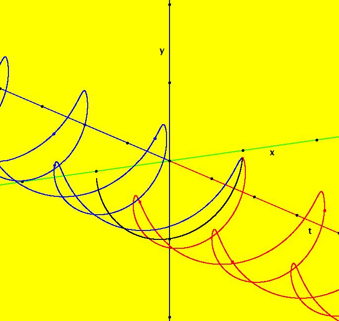
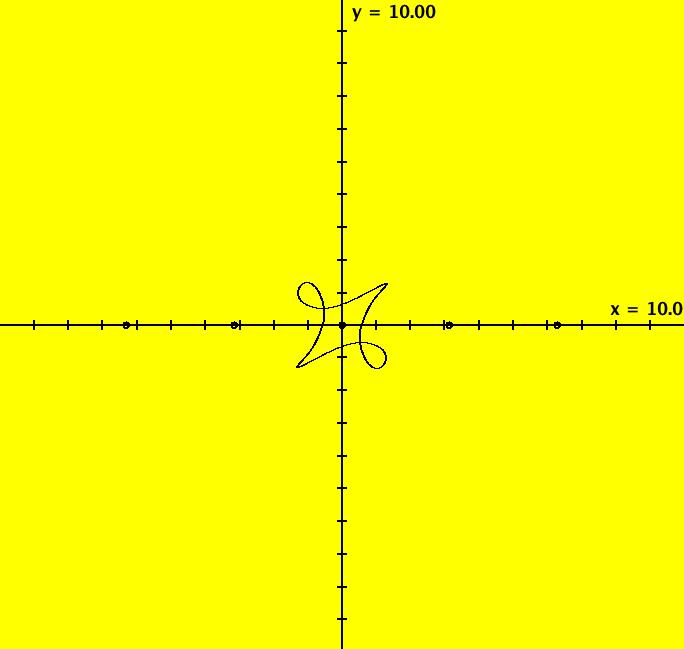
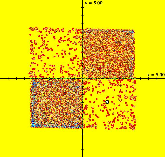
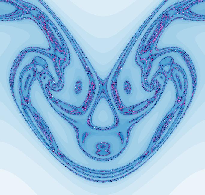
View/Sys/Gal: Ode "ClassicHeliumAtom: Overview" in "PhysicsExs." The Classical Helium Atom Consider the motion of the electrons in the helium atom - neglecting the energy loss due to radiation. The system, which I call the "classical" helium atom, becomes an interesting ode problem, rather than a quantum mechanics problem. To simplify the problem further, I will reduce the number of equations by: (a) starting the two electrons from rest equidistant from the nucleus, (b) assuming that the center of mass of the system is at the nucleus and (c) neglecting the motion of the nucleus. Assumption (b) is justified by noting that the mass of the nucleus is about 10,000 times larger than the mass of the electrons. In the (x,y) coordinate system, let the nucleus be at (0,0) and the two electrons at (x,+-y). By symmetry (assumption (a)), the electrons move in unison in the (x,y) plane on trajectories given by (x(t),y(t)) and (x(t),-y(t)) so only the equation of motion for the electron in the upper half plane is needed. The system is: dx/dt = z, dy/dt = w, dz/dt = -2*x/R, dw/dt = -2*y/R+1/(4*y^2) where R=sqrt(x^2+y^2)^3. The -2*x/R and -2*y/R terms are the components of the attracting force on the electron due to the nucleus and the 1/(2*y)^2 term is the repelling force on the electron due to the second electron. The problem began as a 3-body problem but due to the simplifying assumptions it has been reduced to a 2D 1-body problem of an electron moving in a potential energy well given by: PE(x,y) = -2*(1/sqrt(x^2+y^2)-1/(8*y)) < 0. Plot PE(x,y) in WolframAlpha to see what it looks like. Note that V blows up on the x axis. Using ICs for which: x > 0, y > 0, z = w = 0, the goal is to find, draw and classify the periodic trajectories of the system. All of the systems in this gallery are defined by the same set of odes and the graphics show different periodic trajectories corresponding to different ICs. The ICs were found by searching for approximate periodic trajectories using OdeFactory. See "Q&A 48" in the OdeFactory User Guide for a discussion of why it is not possible for any numerical computation to find and draw exact periodic trajectories. This system was first discussed in the paper: "The Classical Atom Revisited," by J. H. Tutsch, American Journal of Physics, Vol. 38, No. 5, 651-655, May 1970, in which the existence of at least one non-planetary periodic trajectory in the classical model of the n-electron atom was demonstrated.
|
|
|
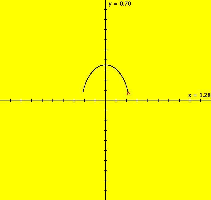
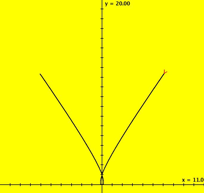
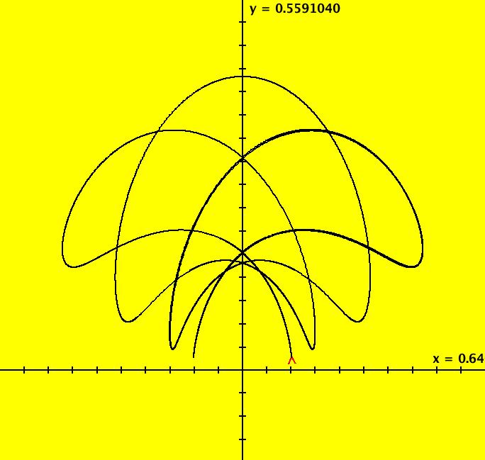
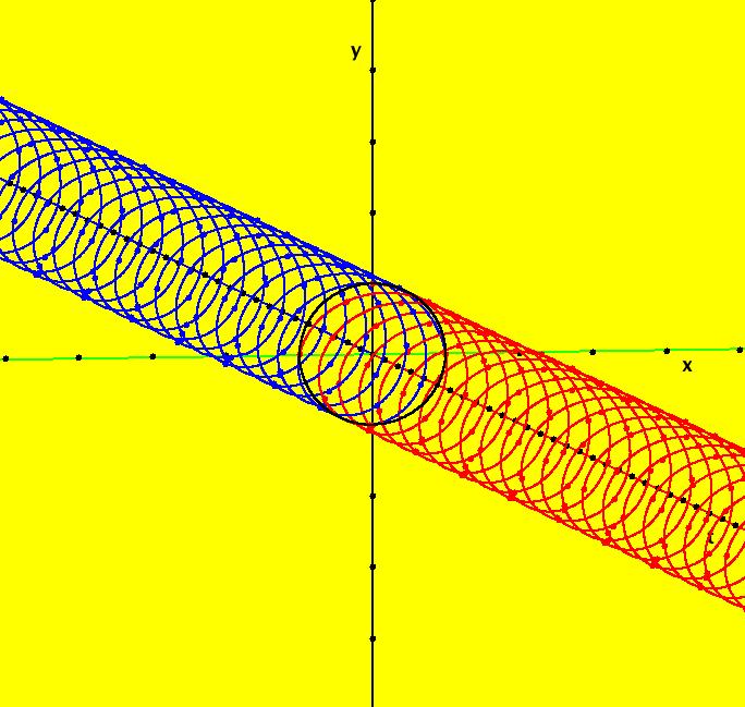
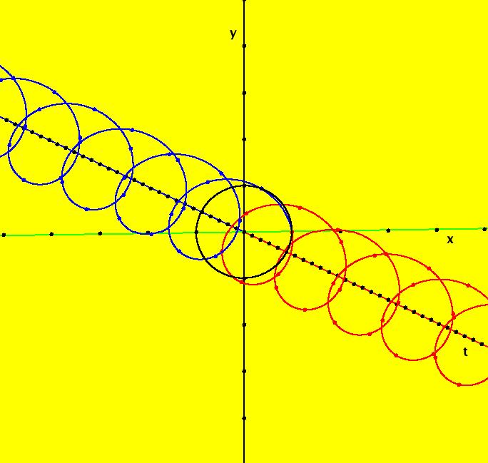
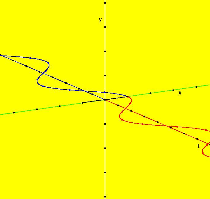
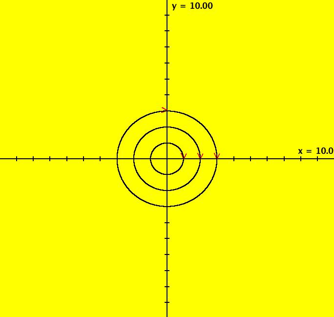
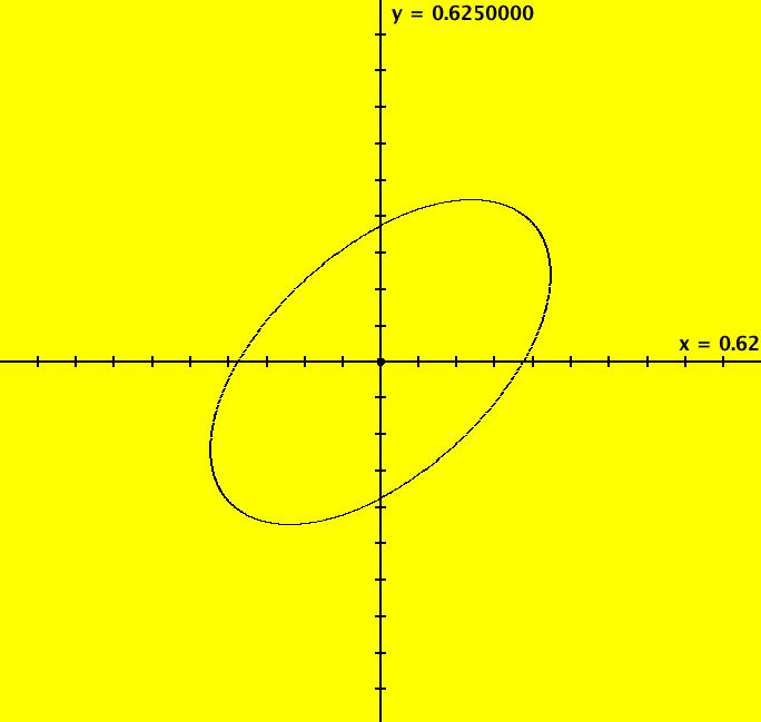
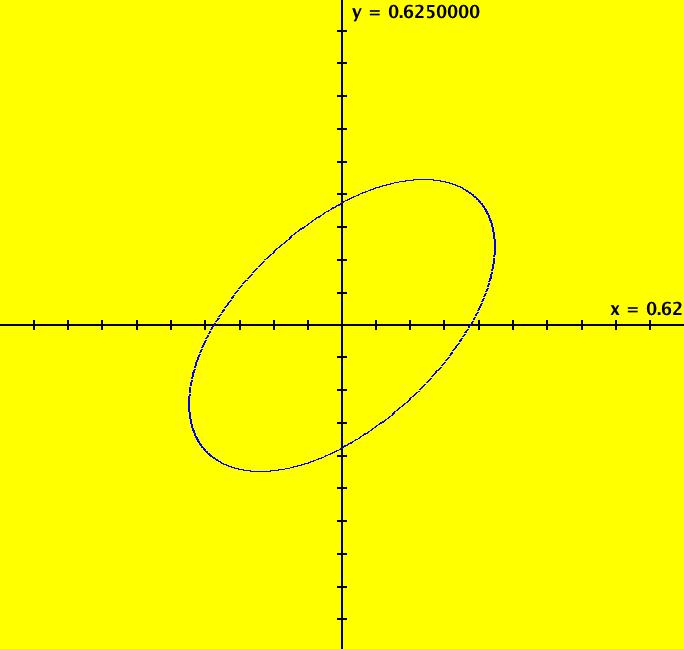
View/Sys/Gal: Ode "ClassicHeliumAtom: 1-0a (x,y,z,w) = (.273212,.058203,0,0)" in "PhysicsExs." The periodic solutions can be classified by their number of y-crossing points and their number of lobes in the first quadrant. A y-crossing point is a point on the y-axis that any part the trajectory crosses twice during one period. A few lines of code were added to OdeFactory, for this gallery only, which mark y-crossing points using red dots. A lobe is a part of a trajectory in the first quadrant connecting any two crossing points. To find a periodic trajectory, start a trajectory in the (x,y) view, in the first quadrant, and watch the location of the red dots as you extend the trajectory in +t. Try to find starting points that produce distinct clusters of red dots. Next refine the starting point by centering on the point and zooming in. Adjust the starting point until the trajectory returns very close to the starting point. 1-crossing trajectories have 0 lobes. There are at least two 1-crossing 0 lobe periodic trajectories. System 1-0a&b shows a second 1-crossing 0 lobe trajectory farther out from the origin. In general, though there seem to be many periodic trajectories for the system, simple periodic trajectories (ones with a low number of y-crossings) are difficult to find. Open questions regarding this system include: - are there an infinite number of trajectories starting at rest on V < 0 that are periodic? - are there an infinite number of trajectories starting at rest on V < 0 that are not periodic? - are all periodic trajectories symmetric about the y axis? - how are the periods related? Image 1: A simple 1-crossing point, 0-lobe trajectory in the (x,y) view. Selecting "Show Approximate Period" on the Settings menu gives the x period of .618. y goes through two small-to-large-to-small cycles in the time it takes x to go through one positive-to-negative-to-positive cycle so the y period is .309. Image 2: 3D/(t,x) view, cycle length = .618. Image 3: 3D/(t,y) view, cycle length = .309.
|
|
|
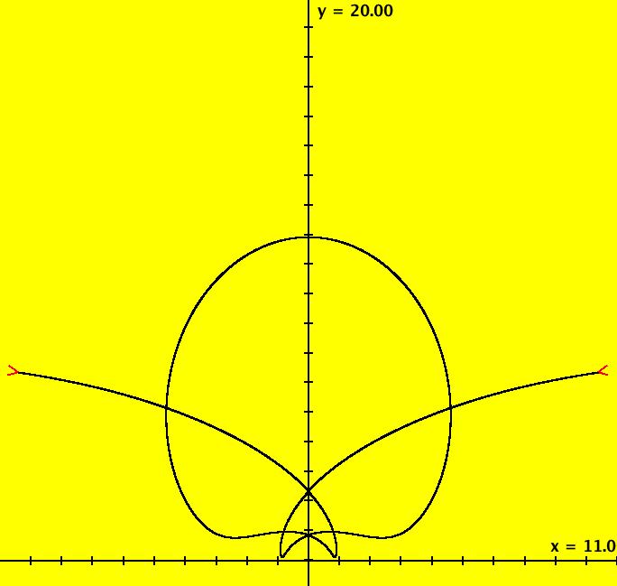
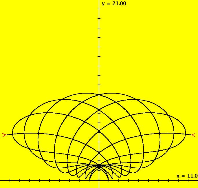
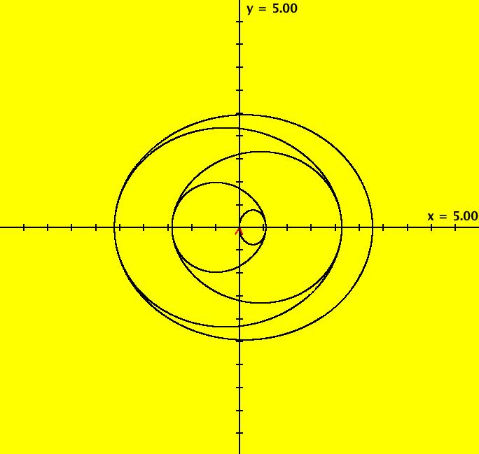
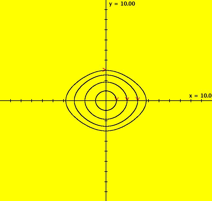
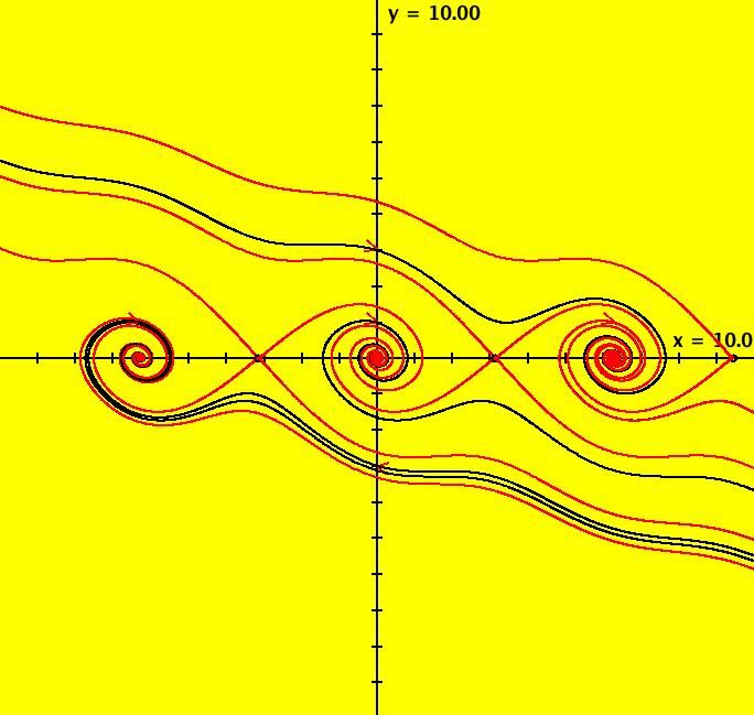
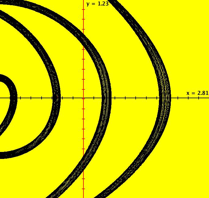
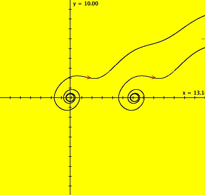
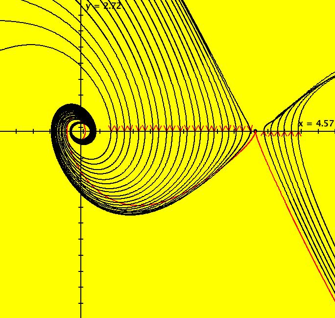
View/Sys/Gal: Ode "ClassicHeliumAtom: 1-0a&b (x,y,z,w) = (6.423387,1.368402,0,0)" in "PhysicsExs." This shows the system 1-0a together with a second 1-crossing 0-lobe periodic trajectory. There are probably many more of these 1-crossing 0-lobe trajectories. Try to find one near (x,y) = (2.4,.5). Try the 3D view. Image 1: Two 1-0 periodic trajectories. The small one is near the origin. The x(t) period of the large trajectory is ~ 71. The x(t) period of the small trajectory is ~ .62.
|
|
|
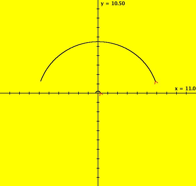
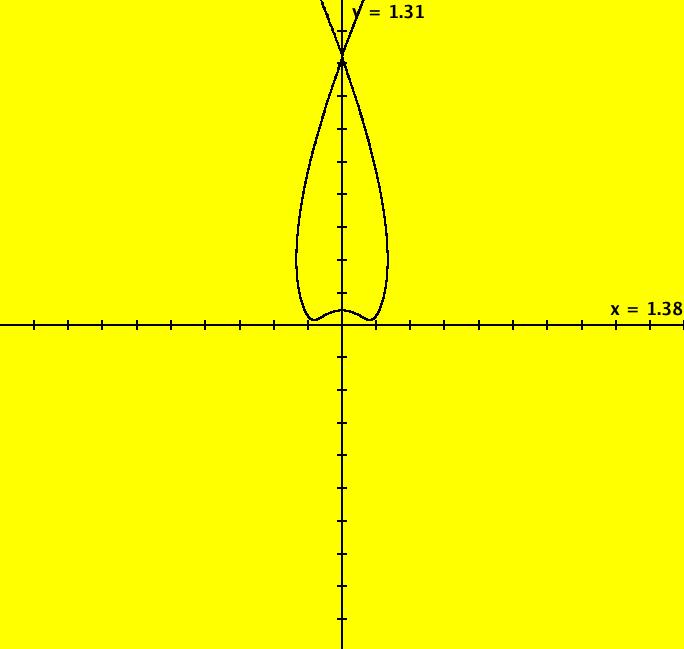
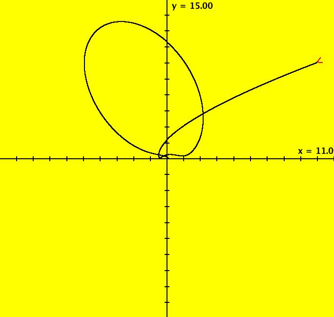
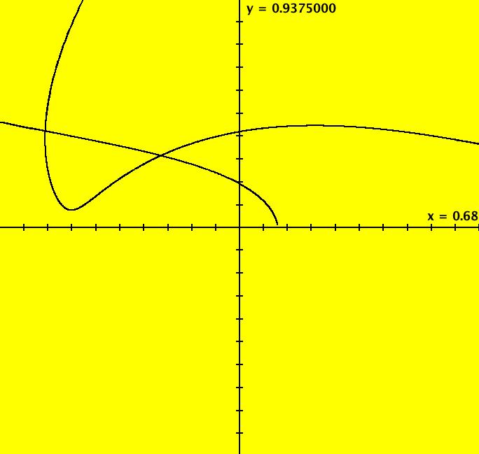
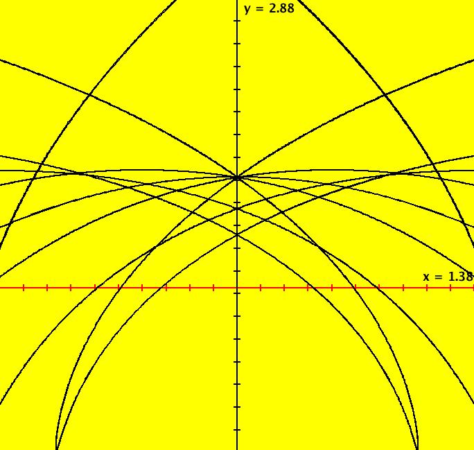
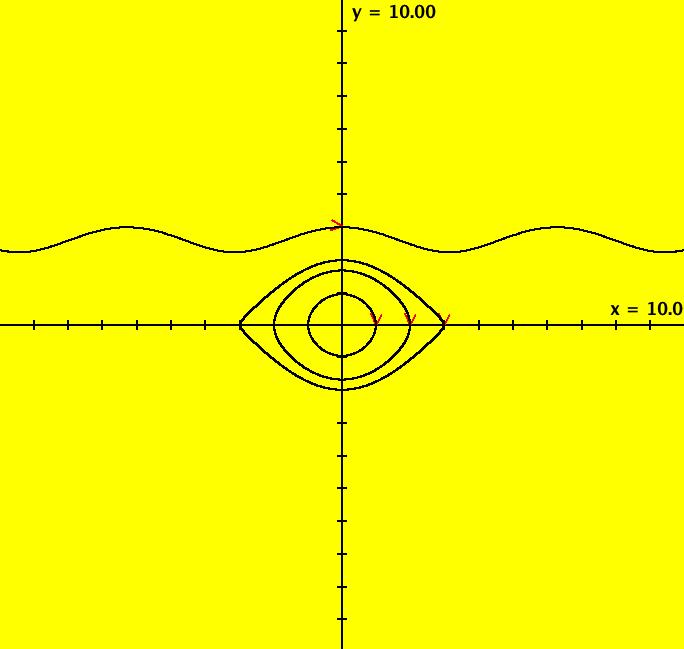
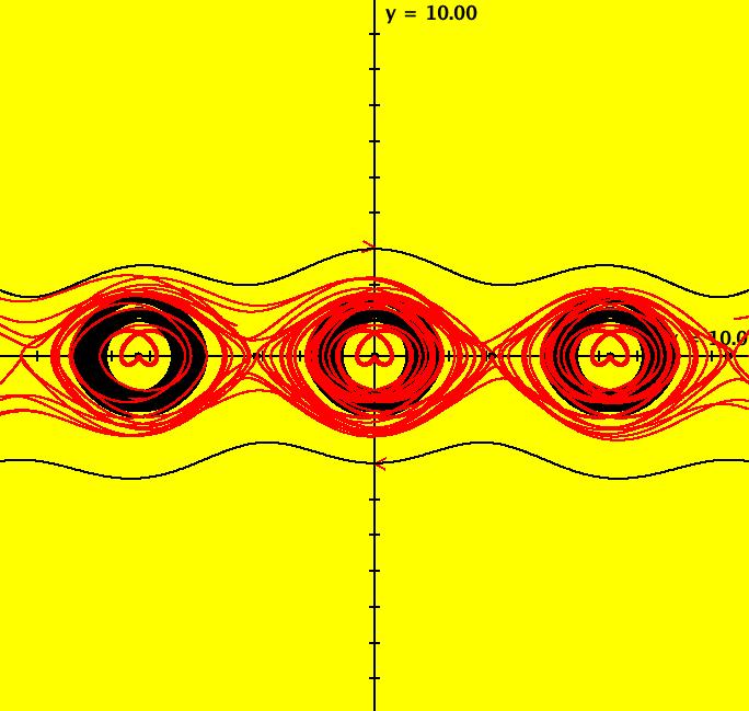
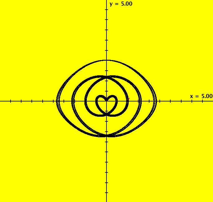
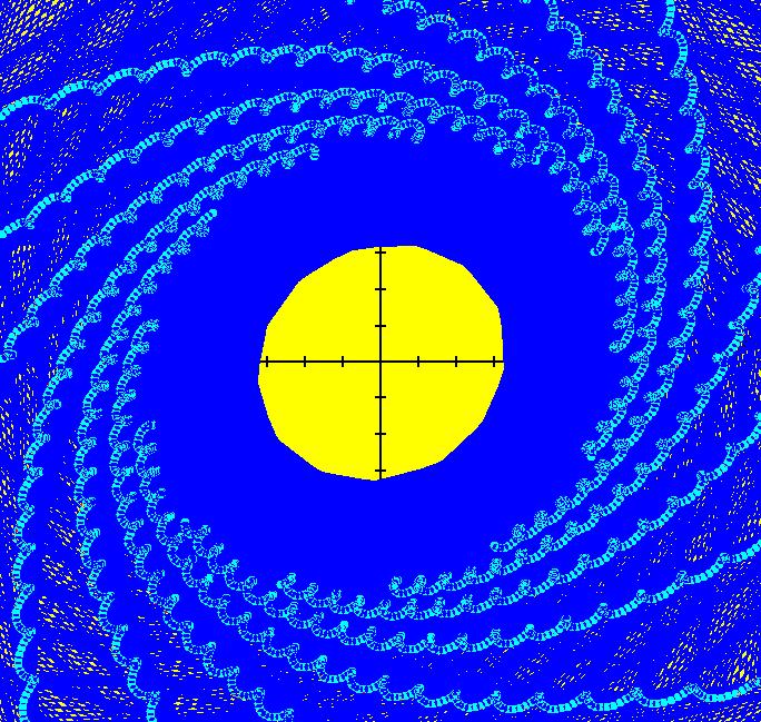
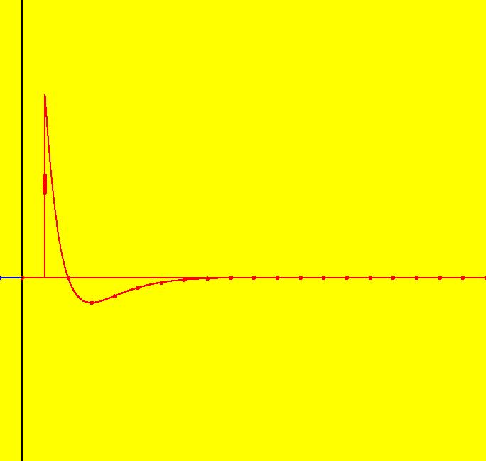
View/Sys/Gal: Ode "ClassicHeliumAtom: 2-1 (x,y,z,w) = (6.672107,11.958786,0,0)" in "PhysicsExs." This is a 2-crossing 1-lobe periodic trajectory. Image 1: A 2-crossing 1-lobe periodic trajectory. The lobe is the part of the trajectory in the first quadrant connecting the two red y-crossing points. Center at the origin and zoom in to see more detail. Image 2: Zoomed-in view centered at (0,0). Near the origin R gets small so dz/dt and dw/dt become large and the motion speeds up.
|
|
|
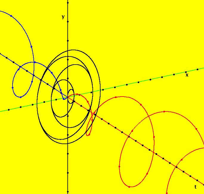
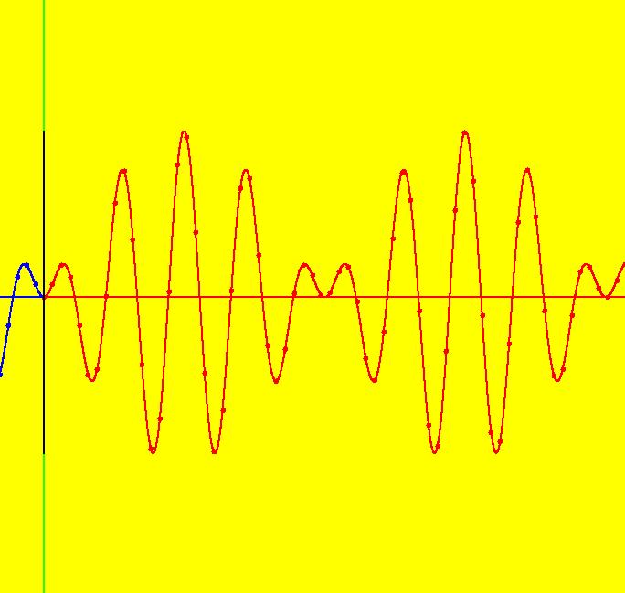
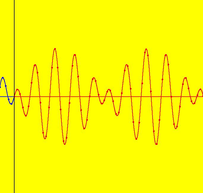
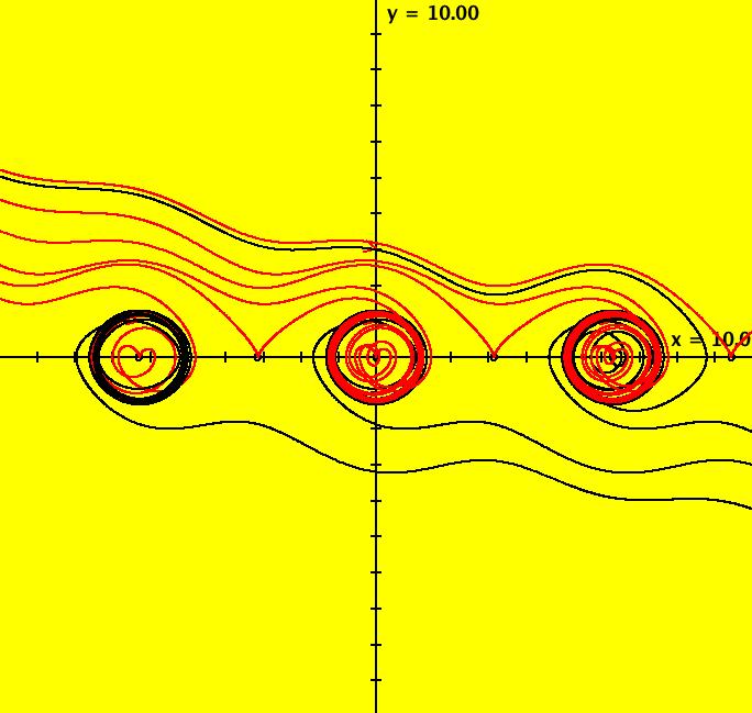
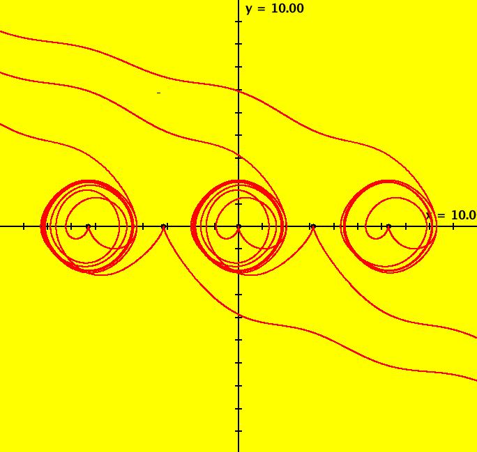
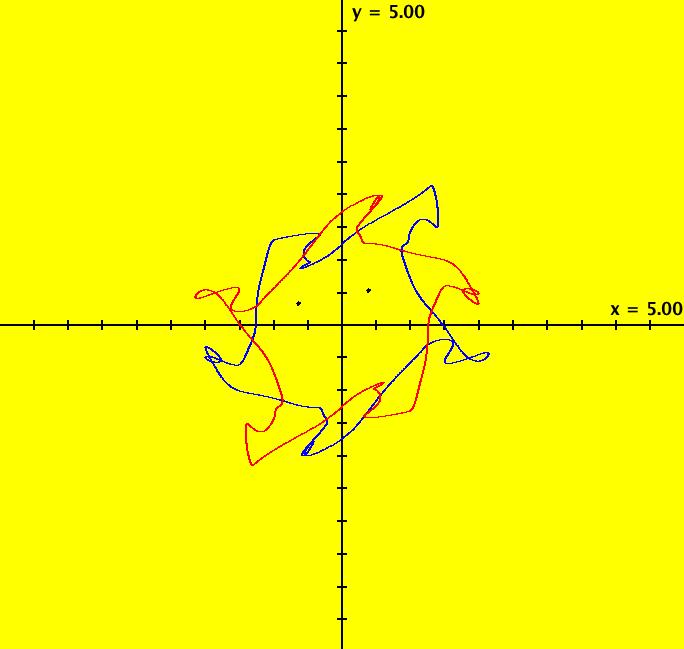
View/Sys/Gal: Ode "ClassicHeliumAtom: 3-2 (x,y,z,w) = (+-10.3000068,6.694971,0,0)" in "PhysicsExs." This is a pair of 3-crossing 2-lobe periodic trajectories that have the same trajectory in the (x,y) view. Image 1: A pair of 3-crossing 2-lobe periodic trajectories. To see the solution curves, zoom out a few times, center near the right end of the x-axis, get into the 3D view and look at the 3D/(t,x) and 3D/(t,y) subviews. Note that if the trajectory starting at (x,y), call it traj1, is periodic then, by symmetry, so is trajectory starting at (-x,y), call it traj2. The 3D/(t,x) view shows that x2(t) = -x1(t) and the 3D/(t,y) view shows that y2(t) = y1(t). Image 2: 3D/(t,x) view. Image 3: 3D/(t,y) view.
|
|
|
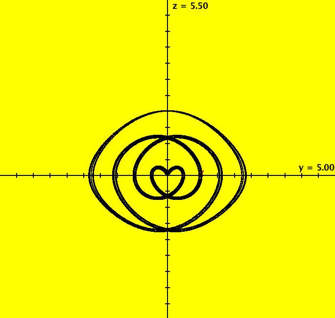
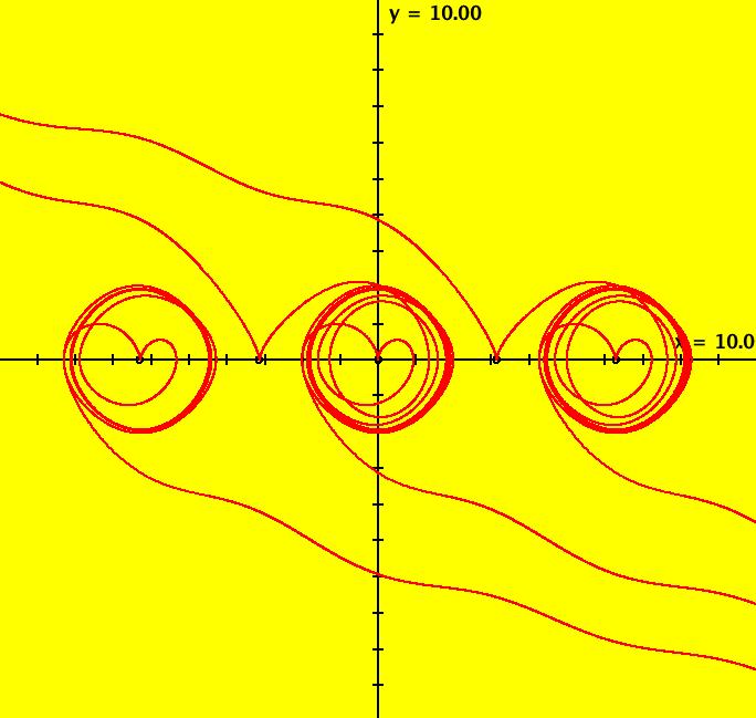
View/Sys/Gal: Ode "ClassicHeliumAtom: 3-3 (x,y,z,w) = (+-9.2,3.37,0,0)" in "PhysicsExs." This is a 3-crossing 3-lobe periodic trajectory. Image 1: A 3-crossing 3-lobe periodic trajectory. There are more n-crossing periodic trajectories but it would take a specialized program to implement a search algorithm to find them. It looks like a trajectory for this system is periodic if it has a perpendicular y-axis crossing so a simple search algorithm would be: (1) pick a curve with potential energy PE(x,y) < 0 and search on the curve in the first quadrant for ICs that produce trajectories that satisfy the "perpendicular y-axis crossing" condition (2) pick a different PE(x,y) < 0 and repeat (1).
|
|
|
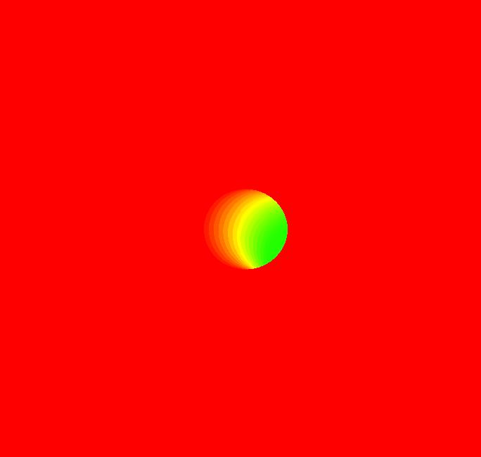
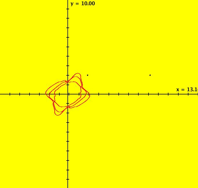
View/Sys/Gal: Ode "ClassicHeliumAtom: 3-? (x,y,z,w) = (9.869223,9.038748,0,0)" in "PhysicsExs." This appears to be a non-symmetric periodic trajectory but it may just seem periodic due to loss of precision in using RK4 near the origin. A stiff solver should be used to study this system further. Image 1: A non-symmetric periodic trajectory? Image 2: Zoomed-in near (0,0).
|
|
|
View/Sys/Gal: Ode "ClassicHeliumAtom: 4-3 (x,y,z,w) = (.130169,.019530,0,0)" in "PhysicsExs." This may be close to a 4-crossing 3-lobe periodic trajectory. Image 1: Ode view.
|
|
|
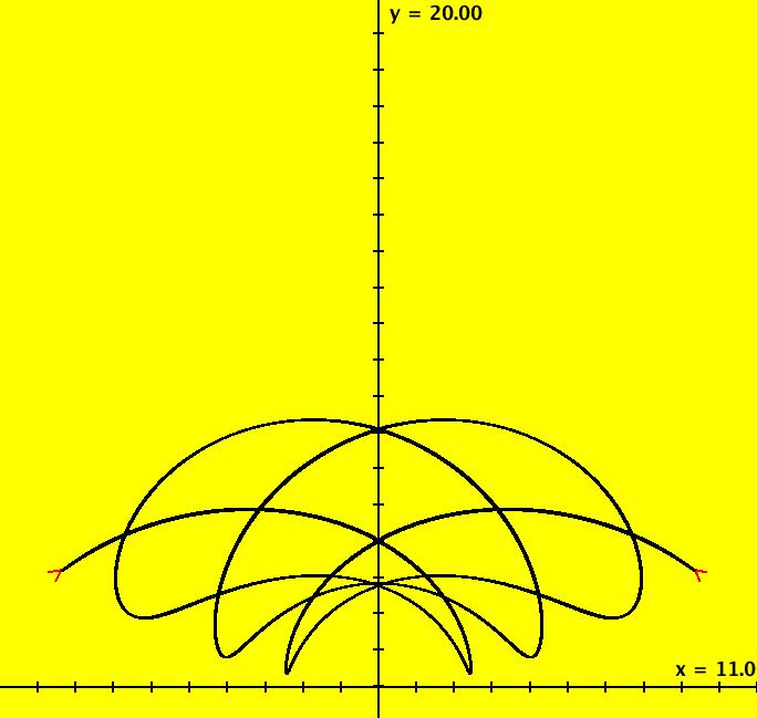
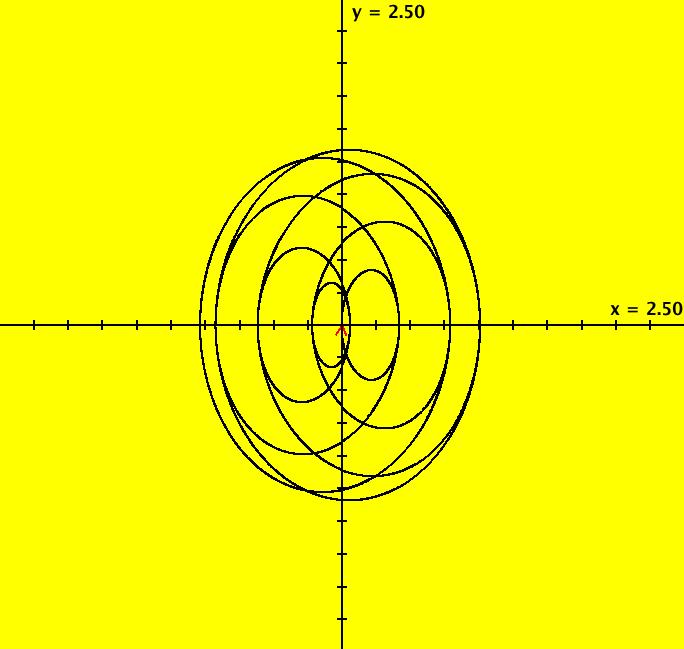
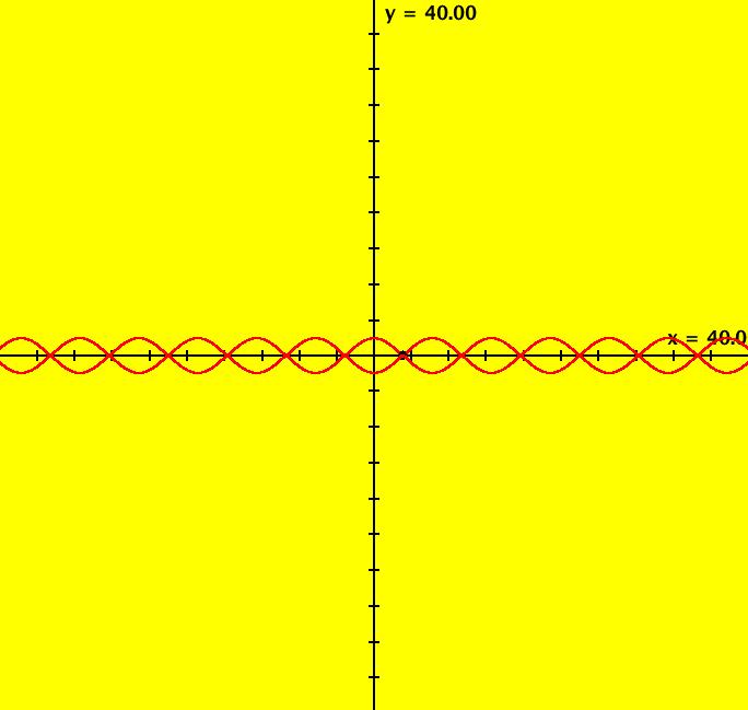
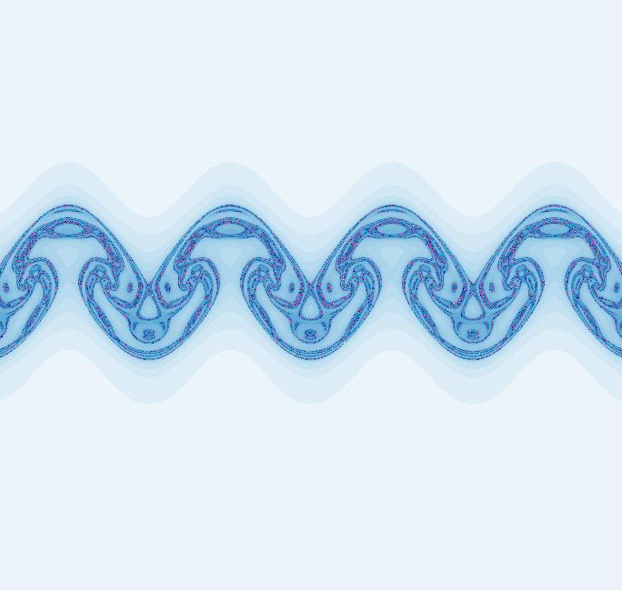
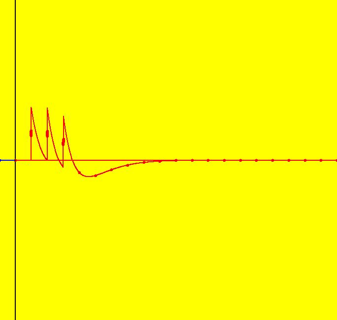
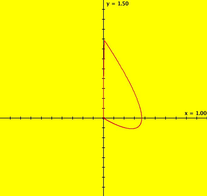
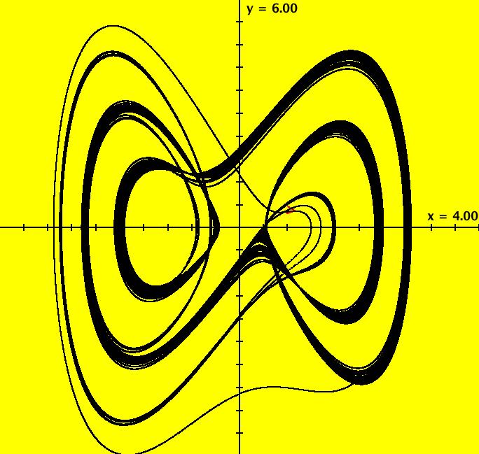
View/Sys/Gal: Ode "ClassicHeliumAtom: 7-8 (x,y,z,w) = (+-10.298,5.28,0,0)" in "PhysicsExs." This is a 7-crossing 8-lobe periodic trajectory. Image 1: A 7-crossing 8-lobe periodic trajectory. It is an example of the non-perpendicular y-crossing case. To see this, center at (0,1.5) and zoom in. Image 2: Zoomed-in at (0,1.5).
|
|
|
View/Sys/Gal: Ode "ClassicHeliumAtom: 7-8 (x,y,z,w) = (+-10.298,5.28,0,0)" in "PhysicsExs." This is a 7-crossing 8-lobe periodic trajectory. Image 1: A 7-crossing 8-lobe periodic trajectory. It is an example of the non-perpendicular y-crossing case. To see this, center at (0,1.5) and zoom in. Image 2: Zoomed-in at (0,1.5).
|
|
An OdeFactory Slide Show Click on a slide to zoom in. Click "video" to see a video. |
View/Sys/Gal: Ode "PendulumExs: Overview" in "PhysicsExs." Pendulum Examples This section contains examples of systems of the form: (A) dx/dt = y, dy/dt = -x and a generalized version of (A), (B) dx/dt = y, dy/dt = -k*sin(x)-c*y+d*sin(t) and a 2nd generalized version of (A), (C) dx/dt = y, dy/dt = -b*y-x+f(t). System (A) models a simple harmonic oscillator (SHO), system (B) models a damped driven pendulum and system (C), discussed in examples (6), models a damped driven SHO or "happiness." System (A) is linear, autonomous and energy conserving. System (B) is nonlinear, nonautonomous, dissipative and driven. System (C) is variations of the SHO. The systems in this gallery are discussed in the Ode, IMap and EMap views.
|
|
|
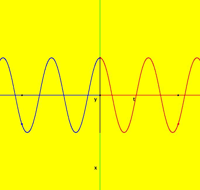
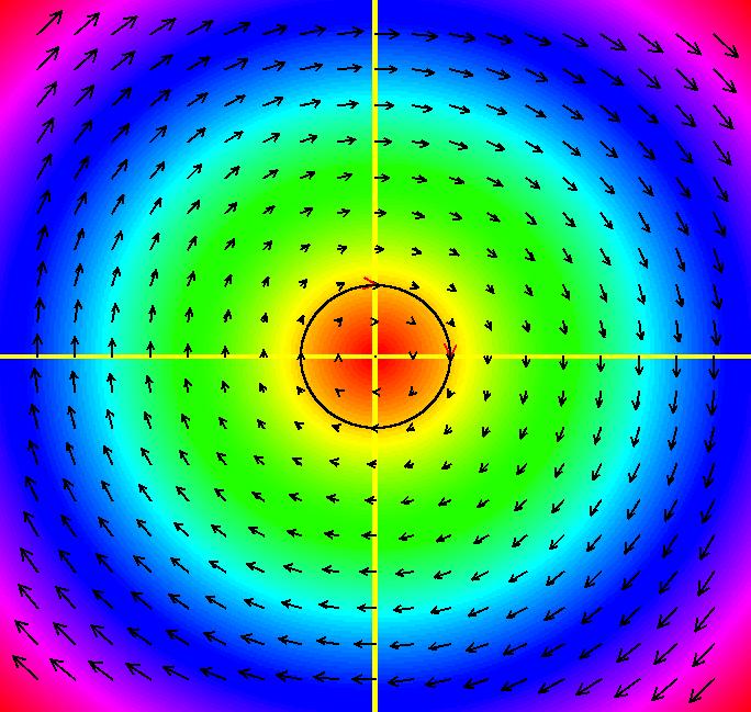
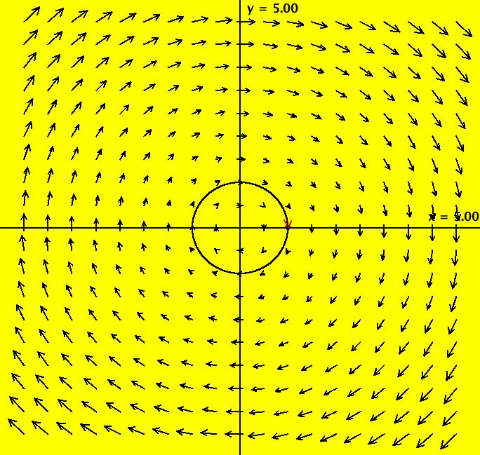
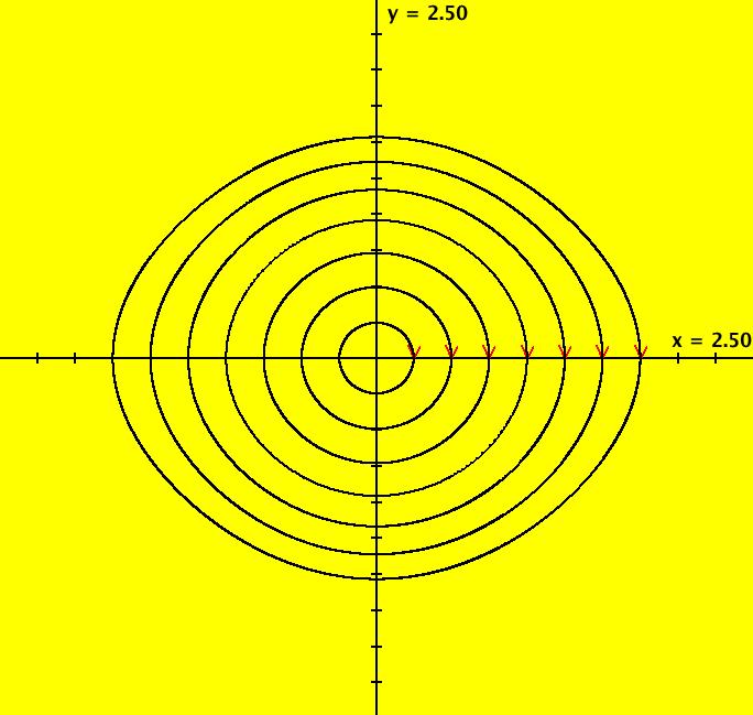
View/Sys/Gal: Ode "PendulumExs: (1.0) (y,-x) SHO" in "PhysicsExs." Simple Harmonic Oscillator (SHO) ~~~~~~~~~~~~~~~~~~~~~~~~~~~~~~~~ This system of odes is defined by the equations: dx/dt = y, dy/dt = -x in the (t,x,y) coordinate system. The 1st order 2D system corresponds to the 2nd order ode y'' = -y in the (x,y,y') coordinate system. This is a 2D linear autonomous system. The vector field is v = (y,-x). Image 1: The colored vector field w/nullclines shown as yellow curves. Linear means the vector field is linear in the state variables x and y. Autonomous means the vector field is constant in t. Math ~~~~ The system can be thought of as the definition of the sin(t) and cos(t) functions. Physics ~~~~~~~ The system can also be thought of as a model of a simple harmonic oscillator, constrained to move in the x direction, examples of which are: - a mass on a spring or - a pendulum where the angle is small. As a 2D, 1st order, system: x(t) is position, y(t) is velocity, dx/dt, and t is time. As a 2nd order ode in normal form: y'' = -y is Newton's law, "F = m*a" where: y is displacement, -y is the external force F, y' is velocity, dy/dx, x is time and y'' is acceleration "a" so F = m*a is -y = m*y''. All physical parameters have been set to 1 in order to focus on the mathematics. --> WA applied to the 1st order system dx/dt = y, dy/dt = -x gives the general solution: x(t) = c_2 sin(t)+c_1 cos(t) y(t) = c_2 cos(t)-c_1 sin(t). WA applied to the normal form version y'' = -y gives the general solution: y(x) = c_2 sin(x)+c_1 cos(x). Note that since the 2D system is equivalent to the normal form equation, y'' = -y, the y(x) solution curve, written in (t,x) coordinates, is the x(t) component of the solution to the 2D system and the y(t) component is just dx(t)/dt. Using he general solution, show that x(t)^2+y(t)^2 = constant, i.e. the trajectories in phase space, (x,y), are circles. You can do the algebra by hand or just apply WA to the expression: simplify (c_2 sin(t)+c_1 cos(t))^2+(c_2 cos(t)-c_1 sin(t))^2 to get c_1^2+c_2^2 so x^2+y^2 is a constant i.e. the trajectories in the phase space are circles. The function H(x,y) = x^2+y^2 = constant is called the Hamiltonian for the system. The constant is the potential energy plus the kinetic energy. H(x,y) is called a "constant of the motion" or an "integral" of the ode. --> Next, find the analytic form of the two solutions satisfying ICs (x,y) = (0,1) and (1,0). by applying WA to the following expression: {x,y}=MatrixExp[{{0,1},{-1,0}}t].{x(0),y(0)} with {x(0),y(0)} = {0,1} then with {1,0}. You should get: solution 1: {x, y} = {sin(t), cos(t)} and solution 2: {x, y} = {cos(t), -sin(t)} Applying WA to dx/dt = y, dy/dt = -x, x(0) = 0, y(0) = 1 and dx/dt = y, dy/dt = -x, x(0) = 1, y(0) = 0 gives the same result. --> Prove that if you advance (i.e. right-shift in time) solution 2 by pi/2 you get solution 1. By applying WA to: {sin(t), cos(t)}={cos(t-pi/2), -sin(t-pi/2)} you get TRUE, so the two solutions are really the same curves. They are just phase-shifted relative to each other. In general, for autonomous systems, all solutions that start on the same trajectory (i.e. the same curve in phase space) differ from each other by a phase shift in the extended phase space. Geometrically they lie on a common surface in the extended phase space. For this system, the surfaces are cylinders about the time axis. --> To see this, start several solutions on the circle of radius 1 then view the solution curves in 3D. Set Yaw = 10, Pitch = 5 and Roll = 0 for a nice view. Image 2: The 3D/(t,x,y) view of 2 solution curves starting on the same trajectory. Click the Flow button to see the "motion" in the phase space. The physical motion of the mass is back and forth on the x axis. It is the projection of the phase space motion in (x,y) onto the the x axis. Using the Flow button on the 4D system (1.1b) system shows the physical motion.
|
|
|
View/Sys/Gal: Ode "PendulumExs: (1.1) (y,-k*x), k=1 SHO w/spring constant" in "PhysicsExs." Use of Control Parameters ~~~~~~~~~~~~~~~~~~~~~~~~~ This system of odes is defined by the equations: dx/dt = y, dy/dt = -k*x in the (t,x,y) coordinate system. Parameters are: k=1 If the system is being used to model a pendulum: x = angular position, y = angular velocity = dx/dt, k = g/d = (2*pi/T)^2 where T = the period, g = 32 ft/sec^2 and d > 0, is the length of the support. If the system is being used to model the motion of a mass on a spring: x = displacement from equilibrium, y = linear velocity = dx/dt and k = c/m = (2*pi/T)^2 where T = period, c is the spring constant and m is the mass. In general, "k" is called a control parameter. Image 1: The vector field and trajectory with k = 1. Image 2: The solution curve in the 3D/(t,x,y) view with k = 1. --> See what happens to the vector field and the trajectory as you vary k from 1 to 2 to -1. --> See what happens to the solution curve, x(t), in the 3D/(t,x) view, as you vary k from 1 to 2 to -1.
|
|
|
View/Sys/Gal: Ode "PendulumExs: (1.1b) (z,0,-k*x,0), k=1 SHO in physical space" in "PhysicsExs." Systems (1.0) and (1.1) model the SHO in the abstract (x,y) phase space where x is the position of an object and y is the object's velocity. The "motion" in (1.0) and (1.1) shows how x and dx/dt change together in time but it does not show directly how the actual physical position of the object changes on the x axis. To see the physical motion we need to go to a 4D version of the system. An object with mass = 1 sitting on the x axis is acted on by a force in the x direction equal to -k*x. The net force in the y direct is zero. Assuming there is no loss of energy due to friction, the Hamiltonian for the system is: H = KE + PE = z^2/2+k*x^2/2. where z is the velocity in the x direction. So dx/dt = ∂H/ ∂z = z, (1) dy/dt = ∂H/ ∂y = 0, (2) dz/dt = - ∂H/ ∂x = -k*x, (3) dw/dt = - ∂H/ ∂y = 0. (4) In the Ode (x,y) view, select "Hide Axes" and start a Flow at max speed for 60 seconds. Watch the object oscillate between x = +-1. Increasing k makes the oscillations faster. Image 1: Ode 3D/(t,x,y) view. You can also get the equations of motion for the system using F=ma. Let x(t) = position of m on the x axis, y(t) = position of m on the y axis, dx/dt = z = velocity in x direction, dy/dt = w = 0 = velocity in y direction, dz/dt = -k*x = force in x direction, dw/dt = 0 = net force in y direction. This is a DAE (differential/algebraic equation) or an ode with a constraint. The constraint is: the table balances the force of gravity. The constraint is applied by setting dw/dt = 0 so dy/dt = 0. ICs for for t = 0 for the trajectory shown are: (x,y,z,w) = (1,0,0,0), or x(0) = 1, force in x dir = -1, y(0) = w(0) = 0, no motion in y dir, z(0) = 0, m starts at rest.
|
|
|
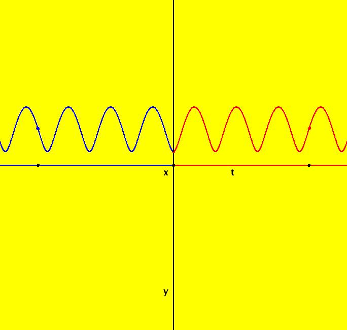
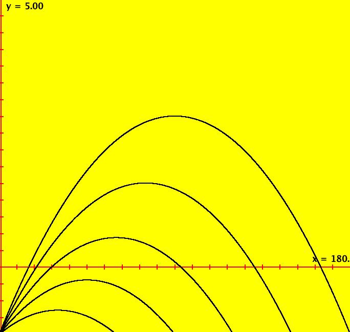
View/Sys/Gal: Ode "PendulumExs: (1.2) (y,-(2*pi/p)^2*x), p = 1.00; period of SHO" in "PhysicsExs." Period of a SHO ~~~~~~~~~~~~~~~ This system of odes is defined by the equations: dx/dt = y, dy/dt = -(2*pi/p)^2*x in the (t,x,y) coordinate system. Parameters are: p = 1.00; The equation of motion for a simple harmonic oscillator is y'' = -(2*pi/p)^2*y where p is the period. For a mass on a spring, p = 2*pi*sqrt(m/c) where m is the mass and c is the spring constant so (2*pi/p)^2 = c/m. For a pendulum with small amplitude, p = 2*pi*sqrt(d/g) where d is the length of the support and g = 32 ft/sec^2 so (2*pi/p)^2 is g/d. Consider a mass on a spring and set the ICs in the 2D (x,y) view to (1,0), (2,0), (3,0). --> Get into the 3D/(t,y) view then set p = 1, 2, 3, 4 and 5 to see if the period is t = 1, 2, 3, 4, 5, as it should be, for each trajectory. Image 1: The 3D/(t,y) view. Another way to see that the period of each trajectory is equal to the value of the parameter p is to select "Show Approximate Period" on the Setting and vary p. --> To learn more about simple harmonic motion, see ... --> To learn more about pendulums, see ...
|
|
|
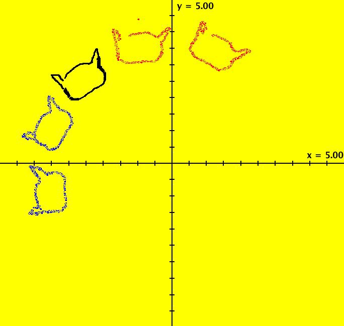
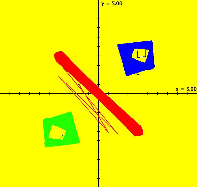
View/Sys/Gal: Ode "PendulumExs: (1.3) (y,-x+k*y), as a map from R2 to R2" in "PhysicsExs." A Vector Field as a Mapping ~~~~~~~~~~~~~~~~~~~~~~~~~~~ This system of odes is defined by the equations: dx/dt = y, dy/dt = -x+k*y or by the vector field v = (y,-x+k*y). The system models a damped linear pendulum when k is not zero. From the geometric point of view, it is sometimes useful to think of the vector field defining a 2D 1st order system of odes as a mapping of R2 into R2. For example, see Arnold's book, "Ordinary Differential Equations. Search in the book for Fig. 107. OdeFactory can be used to animate the action of the mapping in Arnold's cat-face example by drawing a cat face and using the "Flow" button. --> To draw the cat face, Clear the view, select "Hide 2D Ode Trajectories" on the Help menu then, drag out a cat face in the second quadrant. --> Next, startTa Flow with an animation time of 10 seconds. Try k = -.5 then k = .5 then k = 0. --> Watch what happens to the shape of the region defined by the cat face. Image 1: Cat face animation with k = 0 in +t (red) and in -t (blue).
|
|
|
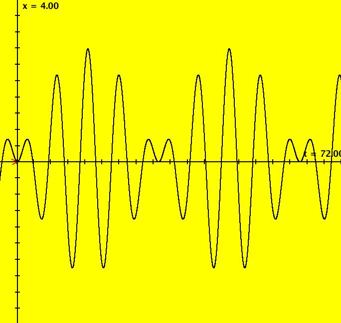
View/Sys/Gal: Ode "PendulumExs: (1.4) (y,-x+d*cos(a*t)), d=.5; a=.8, driven system w/beats" in "PhysicsExs." A Driven Simple Harmonic Oscillator ~~~~~~~~~~~~~~~~~~~~~~~~~~~~~~~~~~~ This is a beat frequency example. The system models the forced vibration of a simple harmonic oscillator without damping. The 2D system of odes is defined by the equations: dx/dt = y, dy/dt = -x+d*cos(a*t) in the (t,x,y) coordinate system. The 1st order 2D system corresponds to the 2nd order ode y'' = -y+d*cos(a*x) in the (x,y,y') coordinate system. Parameters are: d=.5; a=.8 d = coefficient of the driving term a = angular frequency of the driving term = 2*pi/T = 2*pi*f T = the period (sec/cycle) = 1/f f = the frequency (cycles/sec) The forcing function is cos(a*t), which can also be written as sin(a*t+pi/2). The ode is traditionally studied as a 2nd order ode in normal form. Investigate the System Graphically ~~~~~~~~~~~~~~~~~~~~~~~~~~~~~~~~~~ For the trajectory shown in the (x,y) phase space the ICs are (t,x,y) = (0,0,0). The ICs for the solution curves in the (t,x) and (t,y) views have also been set to (0,0,0). Image 1: The phase space, or (x,y), view. --> See the (t,x) and (t,y) views. Image 2: The (t,x) view. Image 3: The 3D/(t,x,y) view w/hMax = 10. Image 4: The 3D/(t,x) view w/hMax = 65. Image 5: The 3D/(t,y) view w/hMax = 65. --> Start a Flow animation at max speed with a duration of 40 seconds. --> In the (x,y) view, check the first six x values corresponding to y = 0. You should get about: x = 0, .54, -1.4, 2.1, -2.6, 2.8. --> In the (t,x) view, check the first six x values corresponding to dx/dt = 0. You should again get about: x = 0, .54, -1.4, 2.1, -2.6, 2.8. To get a better understanding of this system, we need to find the closed form solution for x(t), if possible. Investigate the System Analytically ~~~~~~~~~~~~~~~~~~~~~~~~~~~~~~~~~~~ --> Using WA on dx/dt = y,
dy/dt = -x+d*cos(a*t),
x(0)= 0, y(0) = 0 gives x(t) = (d*(cos(t)-cos(a*t)))/(a^2-1) y(t) = (d*(a *in(a*t)-sin(t)))/(a^2-1). For this 1st order system, y(t) is just dx(t)/dt since the 2D system corresponds to a 2nd order ode in normal form, i.e. y = dx/dt. --> See x(t) in the (t,x) view. To get a better understanding of the system, rewrite x(t) as x(t) = (2*d/(1-a^2))*sin((1-a)/2*t) *sin((1+a)/2*t) where (2*d/(1-a^2)) = the beat amplitude
= max x, (1-a)/2 = the beat frequency. The "natural" frequency of the system is the angular frequency when d = 0, i.e. when there is no driving term. We saw in system (1.0) that the solutions were just linear combinations sin(t) and cos(t) so the "natural" period = 2*pi which makes the natural frequency = 1. In general, the beat amplitude for the driven system is |2*d/((natural freq)^2 -(driving freq)^2)| which goes to infinity as the driving freq goes to the natural freq, which for this example is as "a" goes to +-1. With d = .5 and a = .8 2*d/(1-a^2) = 1/(1-.64) = 2.77778, (1-a)/2 = (1-.8)/2 = .1 and (1+a)/2 = (1+.8)/2 = .9 so x(t) = 2.77778*sin(.1*t)*sin(.9*t) and the beat amplitude = 2.77778 beat period = 2*pi/(beat frequency) = 2*pi/.1 = 20*pi = 62.832 and system period = (beat period)/2 = 10*pi --> Check the beat amplitude, the beat period and the system period in the (t,x) view. --> In the (x,y) view, select "Show Approximate Period" to see that the system period is 2*pi. Normal form Solution vs System Solution ~~~~~~~~~~~~~~~~~~~~~~~~~~~~~~~~~~~~~~~ --> Using WA on the normal form with the parameter values d = .5 and a = .8 and ICs (0,0,0) y'' = -y+.5*cos(.8*x), y(0)=0, y'(0)=0 gives y(x) = 1.38889 cos(0.8 x)-1.38889 cos(x) which can be rewritten as y(x) = 2.77778 sin(.1x)*sin(.9x). --> If you have WA Pro, you can see how WA solves this ode by clicking the "Show steps" button next to the solution in WA. The solution curve, y(x), can be written as x(t) = 2.77778*sin(.1*t)*sin(.9*t). For a 2D system corresponding to a 2nd order ode in normal form, y = dx/dt so, differentiating the expression for x(t) gives, y(t) = 2.5*sin(0.1*t)*cos(0.9*t)+ 0.277778*sin(0.9*t)*cos(0.1*t). WA gives the maximum value for x(t) as 2.77778 and the maximum value for y(t) as 2.46384. See the (x,y) or (t,y) views to check y max. (t,x), (t,y) Views vs 3D/(t,x), 3D/(t,y) Views ~~~~~~~~---~~~~~~~~~~~~~~~~~~~~~~~~~~~~~~~~~~~ For this particular system I have started x(t) and y(t) curves in the (t,x) and (t,y) views using the same ICs as were used for the (x,y) trajectory shown in the (x,t) view. In general, curves started in OdeFactory in different views can have different ICs. For a trajectory started in the (x,y) view, the curves 3D/(t,x) and 3D/(t,y) are projections of the same solution curve in the extended phase space onto the (t,x) and (t,y) planes, i.e. they have the same ICs. --> For a nice 3D view, of the solution curve, return to the original (x,y) view then pan right 4 times, zoom out 2 times and select the t button. --> After scaling by vMax = 4, vMin = -4, hMin = -4, hMax = 72 the 3D/(t,x) view of the trajectory shown is figure 3.9.6, p. 213 from Boyce and DiPrima. Adjusting Parameters ~~~~~~~~~~~~~~~~~~~~ --> Try changing parameter d with "a" fixed. --> Try changing parameter "a" with d fixed. Note what happens as "a" -> +-1. --> Watch the changes in various views. 2D Ode Systems as Iteration Maps ~~~~~~~~~~~~~~~~~~~~~~~~~~~~~~~~ --> Return to the original (x,y) view and click the IMap button. --> Try changing parameter d with "a" fixed. --> Try changing parameter "a" with d fixed. Introduce a Friction Term ~~~~~~~~~~~~~~~~~~~~~~~~~ --> Introduce a velocity dependent friction term, -c*y, into the dy/dt equation. Try to predict what will happen and see what does happen. References ~~~~~~~~~~ Section 3.8, "Mechanical and Electrical Vibrations," of Boyce and DiPrima's classic textbook, "Elementary Differential Equations and Boundary Value Problems," ed. 8, contains a good discussion of the mathematics and physics of beats in driven systems. The system discussed here is example 2, page 212 of the textbook. The figure on the cover of the textbook is the (x,y) view of the trajectory with d = -0.5 and a = 0.9. Google "beat frequency oscillators" for more information.
|
|
|
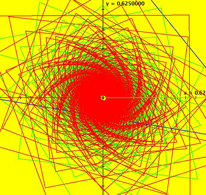
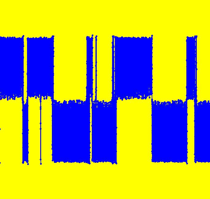
View/Sys/Gal: Ode "PendulumExs: (1.4b) (y,-x+d*cos(a*t)), IMap, d = .810; a = 1.600;" in "PhysicsExs." This iteration is defined by: x <- y, y <- -x+d*cos(a*t). Parameters are: d = .810; a = 1.600; ICs are (x,y) = (0,0). Image 1: An IMap view. --> In the IMap view, try changing parameters d and/or "a." --> Reopen the system with d = .810 and a = 1.6. The EMap view is generated by applying the escape time algorithm to the iterative system. It is most often applied to autonomous polynomial system to produce fractals however in OdeFactory it can be applied to any 2D iterative system. Image 2: An EMap view. --> Go to the EMap view and zoom in. Try changing parameters d and/or "a" again. Image 3: Another EMap view, zoomed in and centered w/CT 2 --> Reopen the system with d = .810 and a = 1.6. --> Go to the Ode view and zoom in. Image 4: The Ode view, zoomed in, periodic trajectory w/period 31.41.
|
|
|
View/Sys/Gal: EMap "PendulumExs: (1.4c) (y,-x+d*cos(a*t)), EMapCT3, d = .810; a = 1.600;" in "PhysicsExs." This iteration is defined by: x <- y, y <- -x+d*cos(a*t). Parameters are: d = .900; a = 1.500; EMap CT: 3 Image 1: Just another interesting EMap view w/CT 3.
|
|
|
View/Sys/Gal: Ode "PendulumExs: (1.5) pendulum motion in physical space" in "PhysicsExs." The previous systems, with the exception of (1.1b), were discussed in the phase space - not the physical space. This system has a 4D phase space but the discussion concerns the observable motion in the 2D (x,y) physical space. The physical motion in the (x,y) plane is subject to the constraint x^2+y^2 = 1 so, for y ≠ 0, dy/dt = -x*dx/dt/y. The system of odes is defined by the equations: dx/dt = z = velocity in x dir, dy/dt = w = velocity in y dir, dz/dt = 32*x*y = force in x dir, dw/dt = -32*x^2 = force in y dir. see: http://math-science.net/?q=node/194 After using the constraint dy/dt = w can be rewritten as dy/dt = -x*z/y for y(t) ≠ 0. Note that for ICs with y(0) < 0, for example (x,y,z,w) = (.994987,-.1,0,0), y(t) stays < 0. Image 1: Ode (x,y) view of the pendulum's path in physical space. Click the Flow button to see the motion in the (x,y) plane. Image 2: Ode 3D/(t,x,y) view of the pendulum's path. Delete the trajectory and start a new one at (x,y,z,w) = (-.7071,-.7071,0,0). Try Flow again. Regarding the y(0) < 0 restriction: If you start a trajectory with y(0) > 0, dy/dt will blow up near y = 0. You could use: dx/dt = -y*w/x and dy/dt = w for y(0) > 0 but the pendulum bob will swing down to x = 0 and dx/dt will blow up. So - this model of a physical pendulum will only work if the pendulum just swings below the x axis. To trick to creating a simulation where the pendulum can swing all the way around is to solve the polar form of the equations of motion: θ'' = -g*sin( θ)/L where r = L <- the constraint goes away! numerically and plot points at (x(t),y(t)) on the circle r = L using values of θ(t) as they are computed.
|
|
|
View/Sys/Gal: Ode "PendulumExs: (2.0) (y,-sin(x)) vs (y,-x)" in "PhysicsExs." ~~~~~~ Approximating sin(x) by x ~~~~~~ This system of odes is defined by the equations: dx/dt = y, dy/dt = -sin(x) in the (t,x,y) coordinate system. These are the correct equations for the pendulum. For small x, sin(x) can be approximated by the first term of its Taylor series which is just x. --> If you don't know the Taylor series for sin(x) at x = 0, apply WA to taylor series for sin(x) at x = 0 or if you never heard of the Taylor series apply WA to approximate sin(x) near x = 0 to get x-x^3/6+x^5/120-x^7/5040+x^9/362880+O(x^10) or, if you just want to keep the difference between sin(x) and x less than 1% apply WA to |x-sin(x)| < .01 to get -.4 < x < .4 --> When does the difference between the approximation of the pendulum system by the following system (the SHO) begin to become noticeable in OdeFactory? dx/dt = y, dy/dt = -x The trajectories start at the x tic marks at intervals of .25 and the trajectories for the approximate system are circles so they would cross the y axis at the y tic marks. The errors show up as the difference between the actual y crossing points and the y tic marks. You can begin to see the difference at about y = .5. Image 1: The y axis crossing points of the trajectories show when approximating -sin(x) by -x begins to make a visible difference. Another way to see the difference is to watch for movement in the vector field as you toggle between the "-sin(x)" and "-x" systems. Try it with systems (2.1) and (2.2).
|
|
|
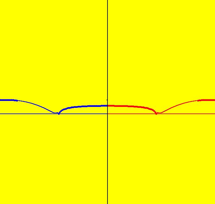
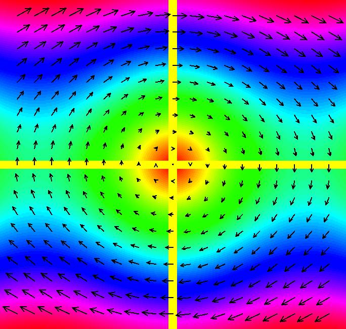
View/Sys/Gal: Ode "PendulumExs: (2.1) (y,-sin(x)) vector field" in "PhysicsExs." ~~~~~~ Approximating sin(x) by x ~~~~~~ This system of odes is defined by the equations: dx/dt = y, dy/dt = -sin(x) in the (t,x,y) coordinate system. These are the correct equations for a simple pendulum. The system is nonlinear and has a complicated solution. --> Apply WA to to the system to find the general solution. --> Toggle between this system and the next one while you watch for slight changes in the vector field in the upper right hand corner. Image 1: The colored vector field using "-sin(x)."
|
|
|
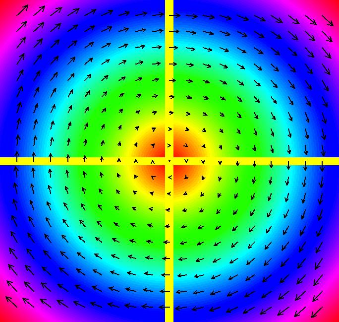
View/Sys/Gal: Ode "PendulumExs: (2.2) (y,-x) vector field" in "PhysicsExs." ~~~~~~ Approximating sin(x) by x ~~~~~~ This system of odes is defined by the equations: dx/dt = y, dy/dt = -x in the (t,x,y) coordinate system. Here x is used to approximate sin(x). The system is linear and has a linear combination of sin(t) and cos(t) for the general solution. Image 1: The colored vector field using "-x."
|
|
|
View/Sys/Gal: Ode "PendulumExs: (2.3) (y,(a-1)*sin(x)-a*x), getting from sin(x) to x" in "PhysicsExs." ~~~~~~ y'' = -sin(y) <---> y'' = -y ~~~~~~ This system of odes is defined by the equations: dx/dt = y, dy/dt = (a-1)*sin(x)-a*x in the (t,x,y) coordinate system. Parameters are: a=0 When a = 0 we have the correct pendulum equations dx/dt = y, dy/dt = -sin(x) and when a = 1 we have the approximate pendulum equations dx/dt = y, dy/dt = -x --> Vary parameter "a" from 0 to 1 and watch the transition from the correct equations to the approximate equations. Image 1: a = 0. Note: when the slider reaches .1, click "Adj Ctrl Params ..." again to open a second parameter controller with a rescaled range. Image 2: a = .5 Image 3: a = 1
|
|
|
View/Sys/Gal: Ode "PendulumExs: (3.0) (y,-sin(x)) drawing a separatrix" in "PhysicsExs." Draw approximate separatrices for the system dx/dt = y, dy/dt = -sin(x). The system has saddle points at odd multiples of pi on the x axis. --> Clear the view and start trajectories at (3.14159, +/-0.0001). Image 1: The separatrix system for the pendulum. Image 2: Zoomed out view to see how well this method works.
|
|
|
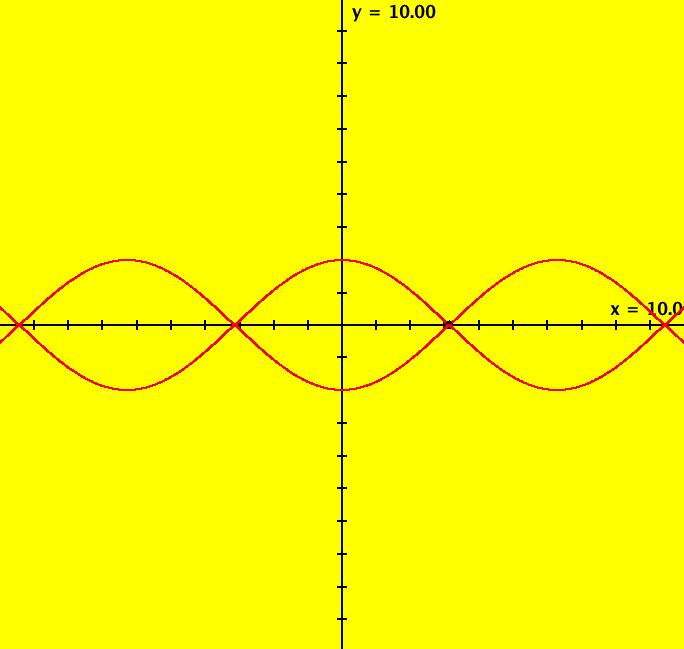
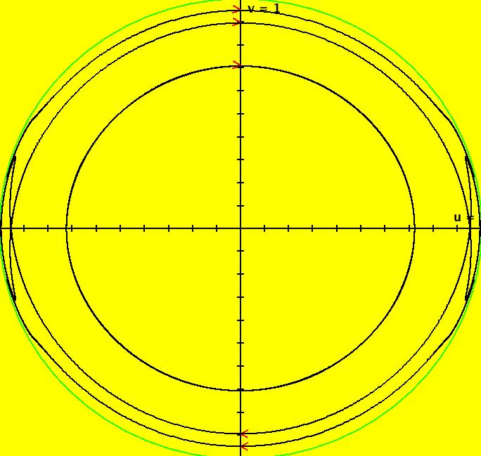
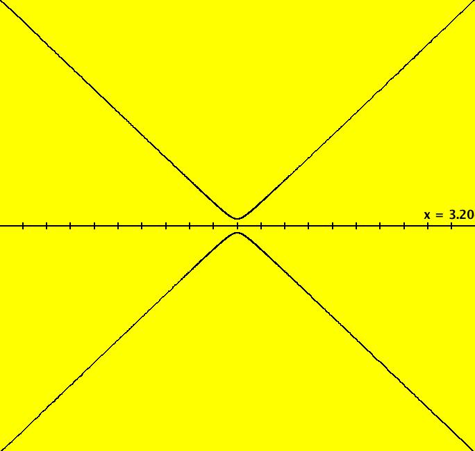
View/Sys/Gal: Ode "PendulumExs: (3.1) (y,-sin(x)), exact separatrices" in "PhysicsExs." This system of odes is defined by the equations: dx/dt = y, dy/dt = -sin(x). Generally it is not possible to find an analytic expression for the separatrices of a nonlinear systems. However the undamped, unforced pendulum is a conservative system with a Hamiltonian function of H = y^2/2 - cos(x). H(x,y) is the total energy of the system and the level curves of H are solution curves of the system (called first integrals). --> Apply WA to y^2/2 - cos(x) to view the level curves of H. The H = 1 level curve corresponds to the separatrices which are the tops and bottoms of the "eyes:" y = +sqrt(2*cos(x)+2) and y = -sqrt(2*cos(x)+2). The finite fixed points are: x = n*pi, n = 0, +-1, etc. The fixed points at infinity are: (u,v) = (+-1,0). --> To see the fixed points at infinity, clear the view, start trajectories above (0,2) and below (0,-2) then switch to R2+. For the phase flow shown, the ICs are: (a) (0,2+-0.000001), approximately on H = 1, give approximate separatrices. Note: Using (0,+-2), which should give the exact separatrices, gives cycles due to the computation errors induced by RK4. (b) (0,1), on H = -.5, gives a cycle. (c) (0,+-3), on H = 3.5, give curves that go to +- infinity. Image 1: The 5 trajectories. Image 2: The R2+ view. Image 3: Image 1 zoomed in at x = pi.
|
|
|
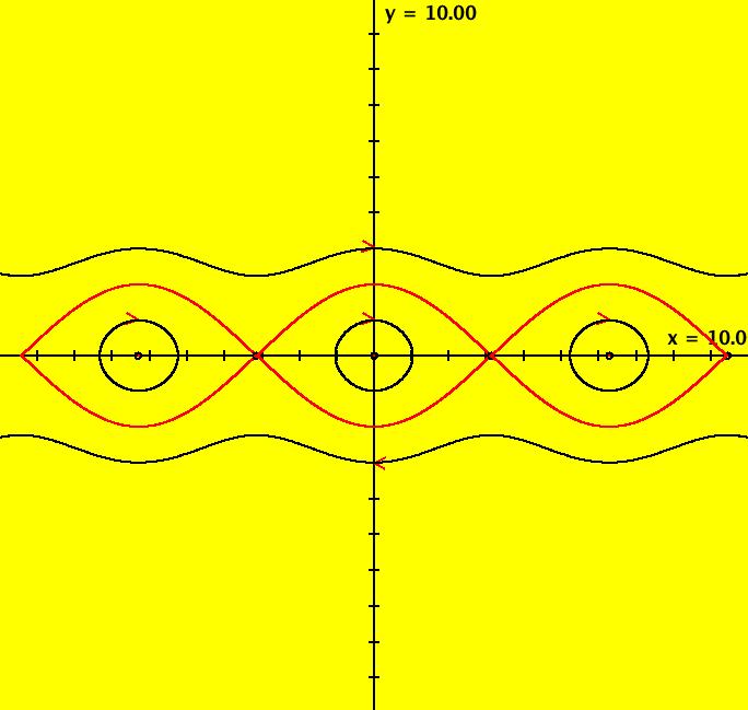
View/Sys/Gal: Ode "PendulumExs: (4.0) (y,-k*sin(x)-c*y+d*sin(t)), k = 1; c = 0; d = 0;" in "PhysicsExs." ~~~~~~ Nonlinear Damped Driven Pendulum ~~~~~~ This system of odes is defined by the equations: dx/dt = y, dy/dt = -k*sin(x)-c*y+d*sin(t) in the (t,x,y) coordinate system. Parameters are: k=1; c=0; d=0 Setting c > 0 turns on the damping term while setting d < 0 turns on the driving term. For d = 0, the fixed points are at x = +-n*pi, where n = 0, 1, 2, ..., and they are shown as small open circles. Points with n = even are centers and points with n = odd are saddle points. ~~~~~~ Drawing a Separatrix ~~~~~~ Separatrices are special isolated trajectories in 2D systems that separate trajectories near saddle points into sets of trajectories that cannot be deformed into each other. In OdeFactory, red trajectories are approximate separatrices. --> To draw the approximate separatrices, start trajectories just to the left and right of the saddle points at +-pi on the x axis. The other ICs correspond to the: 3 center fixed points at (0,0), (+-2pi,0), 3 closed curves at (0,1), (+-2pi,1) and 2 curves going to +-infinity at (0,+-3). Image 1: The undamped, undriven k = 1, c = d = 0 case. For this system, with c = d = 0, the flow in the vertical strip -pi <= x <= pi repeats in the vertical strips from n*pi to (n+2)*pi, where n = +-1, +-3, .... Often the flow on the center strip is mapped to the unit cylinder. The fact that sin(x) = sin(x+n*pi) for n = +-1, +-3, ... causes the repetition. The system in R2 has an infinite number of finite fixed points, two fixed points at infinity and an infinite number of separatrices. The flow on the unit cylinder has two fixed points, one is a center and the other is a saddle, and two separatrices. ~~~~~~ Exploring the Damping and Forcing ~~~~~~ --> Try turning the damping term on by setting k=1; c=.3; d=0, then increase k --> Check out both the Ode and the IMap views. Image 2: Ode view with k = 1, c = .3 and d = 0. In the IMap view, select "Show 2D IMap Orbit Sequence" on the Help menu. Image 3: IMap view zoomed in with k = 1, c = .3 and d = 0 showing the orbit sequence.
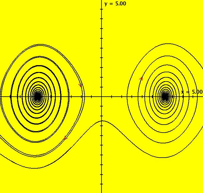
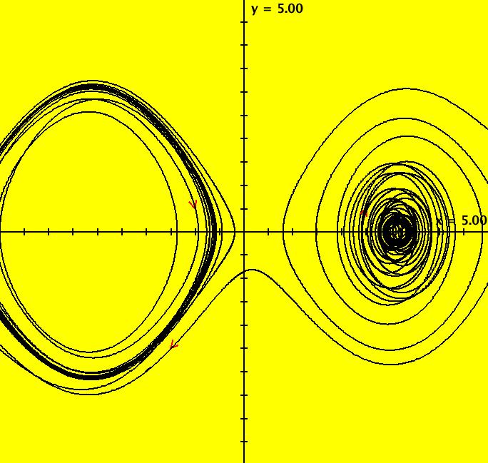
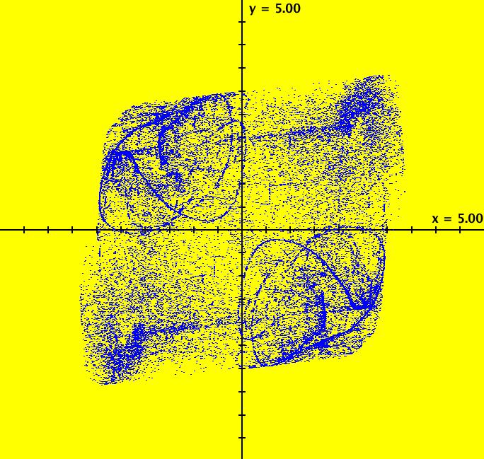
--> In the Ode view, try turning the driving term on by setting k=1; c=0; d=-.3 Image 4: Ode view with k = 1, c = 0 and d = -.3. Image 5: The IMap view, zoomed in, with k = 1, c = 0 and d = -.3 shows a strange attractor. --> Try turning both the damping and driving terms on by first increasing c and then increasing d. Image 6: Ode view with k = 1, c = .2 and d = .3.
|
|
|
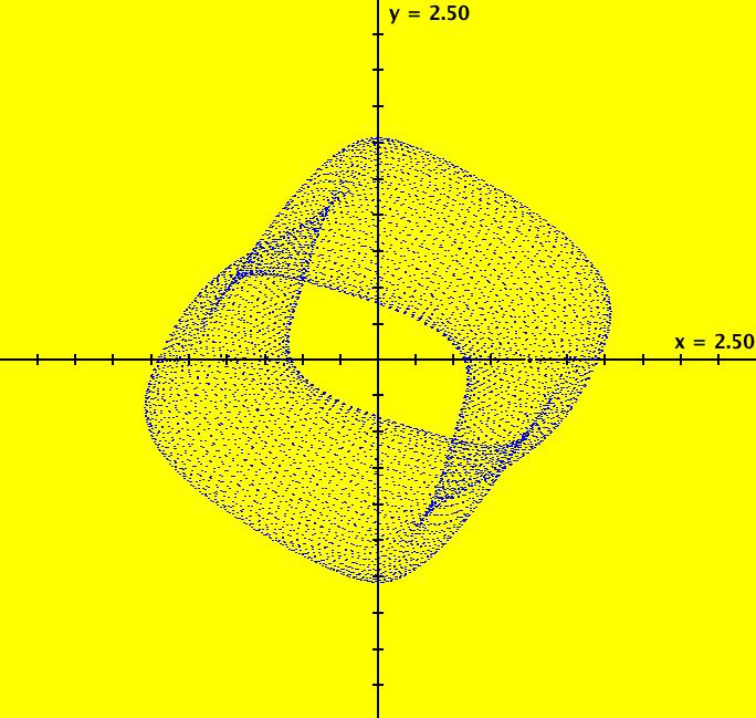
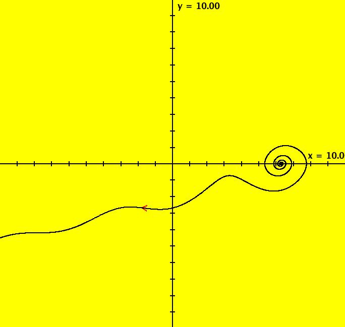
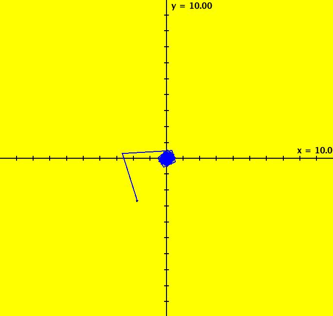
View/Sys/Gal: Ode "PendulumExs: (4.1) (y,-k*sin(x)-c*y+d*sin(t)), 2D nonautonomous k=1; c=0; d=.3" in "PhysicsExs." ~~~~~~ Odes and IMaps ~~~~~~ This 2D nonautonomous system of odes is defined by the equations: dx/dt = y, dy/dt = -k*sin(x)-c*y+d*sin(t) in the (t,x,y) coordinate system. Parameters are: k=1; c=0; d=.3 ICs are (t,x,y) = (0,1,0) Image 1: The Ode view. ~~~~~~ An Ode as an IMap (Iterative Map) ~~~~~~ --> Toggle the IMap button to get to the "IMap" view where you will see the 2D iterative map defined by the system. Image 2: The IMap view. To see if the trajectory is periodic, for d = .3, alt-click on the arrowhead to center the view at the origin then zoom in to view the trajectory in more detail. Extend the trajectory in +t. Image 3: A zoomed in Ode view with the trajectory extended in +t.
|
|
|
View/Sys/Gal: Ode "PendulumExs: (4.1b) (1,z,-k*sin(y)-c*z+d*sin(x)), 3D autonomous k=1; c=0; d=.3" in "PhysicsExs." This is the 3D autonomous version of the 2D nonautonomous system (4.1). This system of odes is defined by the equations: dx/dt = 1, dy/dt = z, dz/dt = -k*sin(y)-c*z+d*sin(x). Parameters are: k=1; c=0; d=.3 In the (y,z) view, the ICs are: (t,x,y,z) = (0,0,1,0). The +x axis is into the screen and the screen is the x = 1 plane. The initial point, (y,z) = (1,0) corresponds to the initial point in system (4.1) of (x,y) = (1,0). In both cases t0 = 0. Image 1: The Ode view in the (y,z) plane with x = 1. The algorithm for the conversion from the 2D nonautonomous system to the 3D autonomous system basically involves "promoting" time to a state variable. Starting with: dx/dt = y, dy/dt = -k*sin(x)-c*y+d*sin(t) where x(1) = x, x(2) = y and x(3) = z, for (j = 2 to 1) { for (i = 2 to 1) { // promote x(i) to x(i+1) in RHS(j), x(i) -> x(i+1) } // promote t to x(1) in RHS(j), t -> x(1) // promote ode(j) to ode(j+1) dx(j+1)/dt = RHS(j) }
prepend dx(1)/dt = 1 to get dx/dt = 1, dy/dt = z, dz/dt = -k*sin(y)-c*z+d*sin(x).
|
|
|
View/Sys/Gal: IMap "PendulumExs: (5.0) (y,-k*sin(x)-c*y+d*sin(a*t)), IMap, w/attractor" in "PhysicsExs." ~~~~~~ 2D Odes as Iterative Maps ~~~~~~ This system of odes is defined by the equations: dx/dt = y, dy/dt = -k*sin(x)-c*y+d*sin(a*t) in the (t,x,y) coordinate system. Parameters are: k=1.2; c=.3; d=.8; a=.2 ICs are (1,0). This nonautonomous 2D system generates interesting iterative maps, most 2D odes (autonomous or nonautonomous) do not. As an iteration map the system is: x <- y, y <- -k*sin(x)-c*y+d*sin(a*t) i.e. the t step size, | Δt|, is 1. The "+t" part of the iteration uses Δt = 1. OdeFactory does not implement a "-t" IMap iteration, i.e. it does not draw an inverse iteration. Image 1: IMap view with parameters k=1.2; c=.3; d=.8; a=.2 --> Vary the parameters. --> Zoom out once then try k = -1.6, c = .1, d = 1.3 and a = -3.2. Switch to the Ode view again. Image 2: IMap view zoomed out with parameters k = -1.6, c = .1, d = 1.3 and a = -3.2 Image 3: EMap view with k = -1.6, c = 1, d = .8 and a = .2 --> For additional interesting 2D map examples, see system "Ode/IMap/EMap" in gallery OdeFactoryExs.
|
|
|
View/Sys/Gal: IMap "PendulumExs: (5.0b) (y,-k*sin(x)-c*y+d*sin(a*t)), IMap, w/attractor" in "PhysicsExs." This system of odes is defined by the equations: dx/dt = y, dy/dt = -k*sin(x)-c*y+d*sin(a*t) in the (t,x,y) coordinate system. The 1st order 2D system corresponds to the 2nd order ode: y'' = -k*sin(y)-c*y'+d*sin(a*x) in the (x,y,y') coordinate system. Parameters are: k = 1.200; c = .380; d = .850; a = -1.000; ICs: (x,y) = (+-n*pi,0), n = 0, 1, 2 Image 1: IMap view with a single attractor. Image 2: Ode view with a = -1 and ICs (x,y) = (+-n*pi,0) for n = 0, 1, 2. There are an infinity of attractors in the Ode view. Image 3: Ode view with a = 1.
|
|
|
View/Sys/Gal: Ode "PendulumExs: (5.1) (y,-k*sin(x)-c*y+d*sin(t)), IMap, w/attractor" in "PhysicsExs." This iteration is defined by: x <- y, y <- -k*sin(x)-c*y+d*sin(t). Parameters are: k = 1.500; c = -.500; d = .280; This is a 2D non-autonomous system. The object that looks like a curve is made up of dots. It is an attractor for the IMap. ICs are (x,y) = (2,2) and (2+2*pi,2) Image 1: IMap view. --> Start a flow. --> Go to the Ode view. In the Ode view there are an infinite number of attractors in -t. They are α-limit sets. Image 2: Ode view with two α-limit sets shown. --> Vary the parameters.
|
|
|
View/Sys/Gal: IMap "PendulumExs: (5.1b) (y,-k*sin(x)-c*y+d*sin(t)), IMap, w/two attractors" in "PhysicsExs." This iteration is defined by: x <- y, y <- -k*sin(x)-c*y+d*sin(t). Parameters are: k = 1.500; c = -.500; d = .320; In the IMap view, this seems to be two different attractors. Rotating one curve by 180 degrees gives the other curve. Image 1: IMap view. --> Add more seeds to see what happens.
|
|
|
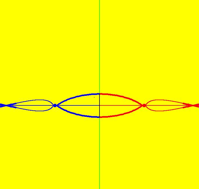
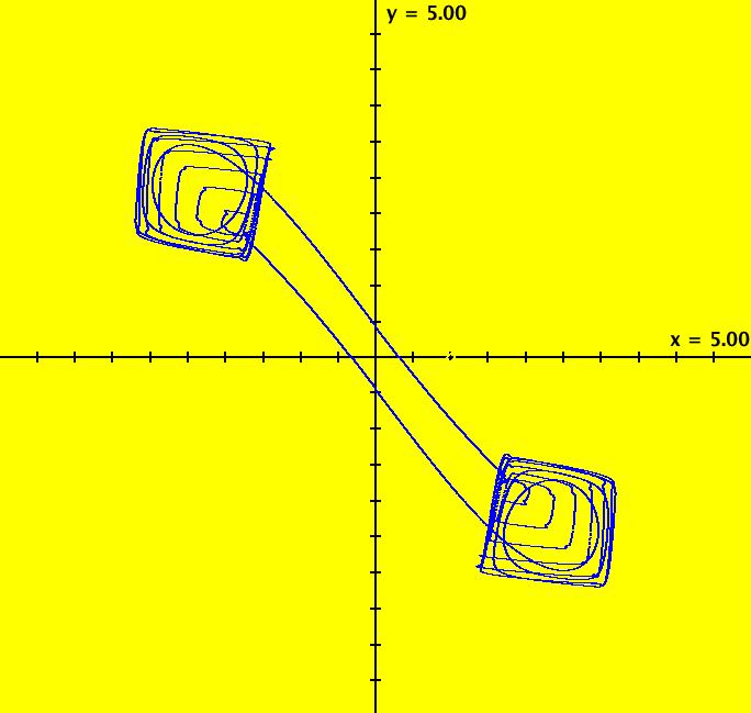
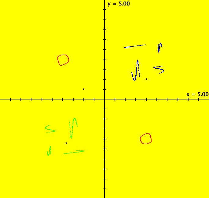
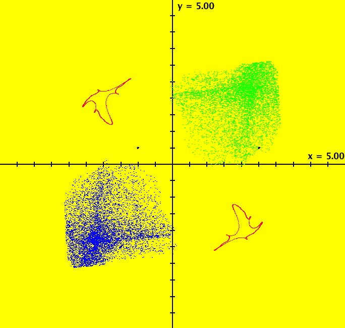
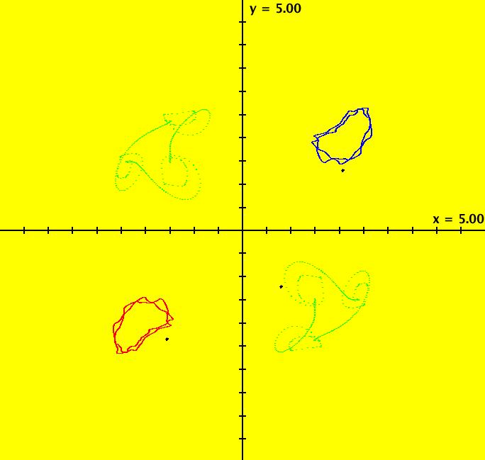
View/Sys/Gal: Ode "PendulumExs: (5.1c) (y,-k*sin(x)-c*y+d*sin(t)), IMap, w/three attractors" in "PhysicsExs." This iteration is defined by: x <- y, y <- -k*sin(x)-c*y+d*sin(t). Parameters are: k = -2.500; c = -.120; d = .000; Note that with d = 0 this is really a 2D autonomous system. There seems to be two disjoint, but symmetric, attractors in the first and third quadrants and a single attractor with parts in the second and fourth quadrants. ICs: (x,y) = (2,1) blue, (-1,.5) red and (-1.8,-2.2) green. Image 1: IMap view. Image 2: IMap view with orbit sequence. Image 3: Ode view. --> Try adding more seeds.
|
|
|
View/Sys/Gal: IMap "PendulumExs: (5.1d) 2D nonauton -> 3D auton" in "PhysicsExs." The three systems (5.1d) are a bit of an aside. The point is to show how a nonautonomous 2D system can be converted to an autonomous 3D system by "promoting" time to a state variable. See gallery NonAutonToAutonExs for a detailed description of the algorithm. This iteration is defined by: x <- y, y <- -k*sin(x)-c*y+d*sin(t). Parameters are: k = -2.500; c = -.090; d = .370; ICs: (x,y) = (-1.5,-2.5), (-1,.5), (2.5,.5). Image 1: Ode view. Image 2: IMap view.
|
|
|
View/Sys/Gal: IMap "PendulumExs: (5.1d) 3D auton IMap-equivalent, different ode" in "PhysicsExs." This system of odes is defined by the equations: dx/dt = x+1, dy/dt = z, dz/dt = -k*sin(y)-c*z+d*sin(x). Parameters are: k = -2.500; c = -.090; d = .370; ICs: (x,y,z) = (0,-1.5,-2.5), (0,-1,.5), (0,2.5,.5). The Ode view is NOT the same as the Ode view of the previous 2D nonauton system. Note: to get to the Ode view of this system you need to delete IMap from the system's name, then reopen the system. Image 1: The IMap view, same as the IMap view of the 2D nonauton system.
|
|
|
View/Sys/Gal: Ode "PendulumExs: (5.1d) 3D auton Ode-equivalent, different imap" in "PhysicsExs." This system of odes is defined by the equations: dx/dt = 1, dy/dt = z, dz/dt = -k*sin(y)-c*z+d*sin(x). Parameters are: k = -2.500; c = -.090; d = .370; ICs: (x,y,z) = (0,-1.5,-2.5), (0,-1,.5), (0,2.5,.5). Image 1: The Ode view, the same as the Ode view of the 2D nonauton system. The IMap view is NOT the same as the IMap view of the 2D nonauton system. Note: to get to the IMap view of this system you need to replace Ode in the system's name, then reopen the system.
|
|
|
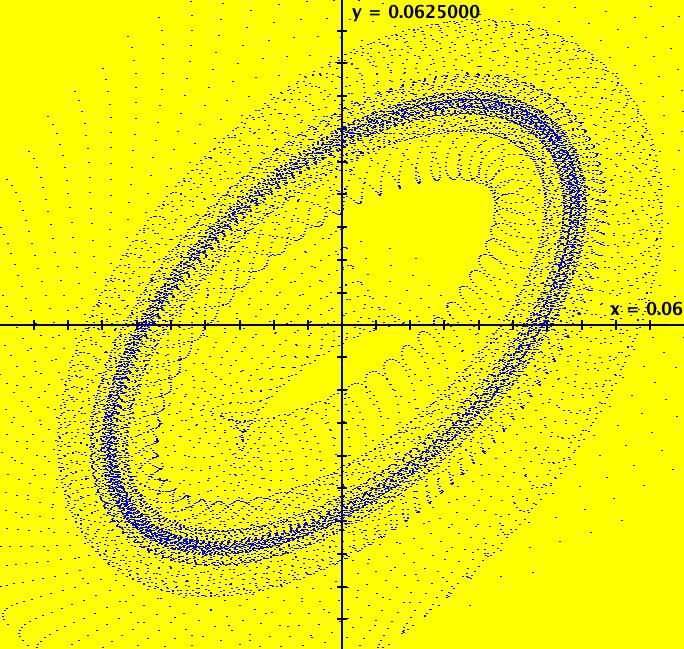
View/Sys/Gal: IMap "PendulumExs: (5.1e) (y,-k*sin(x)-c*y+d*sin(t)), IMap, k = 1.000; c = -.240; d = -.001;" in "PhysicsExs." This iteration is defined by: x <- y, y <- -k*sin(x)-c*y+d*sin(t). Parameters are: k = 1.000; c = -.240; d = -.001; --> Try an animation at max speed for 30 sec. Image 1: After 30 sec animation, at .125 by .125. --> Select "Show 2D IMao Orbit Sequence" on and do it again. Image 2: After 30 sec animation w/orbit sequence on, at .125 by .125. Image 3: The Ode view at 20 by 20. Image 4: The IMap view at 20 by 20. Ode trajectories fill the phase space while IMap orbits live near the origin.
|
|
|
View/Sys/Gal: IMap "PendulumExs: (5.1f) (y,-k*sin(x)-c*y+d*sin(t)), IMap, k = 1.000; c = -.140; d = -.040;" in "PhysicsExs." This iteration is defined by: x <- y, y <- -k*sin(x)-c*y+d*sin(t). Parameters are: k = 1.000; c = -.140; d = -.040; --> Adjust the parameters to see what happens. Image 1: Another interesting IMap orbit. --> Try a Flow animation. --> Add some seeds.
|
|
|
View/Sys/Gal: IMap "PendulumExs: (5.1g) (y,-k*sin(x)-c*y+d*sin(t)), IMap, k = -3.100; c = .030; d = .034;" in "PhysicsExs." This iteration is defined by: x <- y, y <- -k*sin(x)-c*y+d*sin(t). Parameters are: k = -3.100; c = .030; d = .034; This IMap is an oscillating strange attractor. --> Start an animation at max speed for 60 sec to see the oscillation. Image 1: IMap view after a 60 sec animation. Image 2: IMap 3D/(t,x) view with hMin = 0, hMax = 10000. --> Try adjusting the parameters.
|
|
|
View/Sys/Gal: IMap "PendulumExs: (5.1h) (y,-k*sin(x)-c*y+d*sin(t)), IMap, k = -2.500; c = -.120; d = .510;" in "PhysicsExs." This iteration is defined by: x <- y, y <- -k*sin(x)-c*y+d*sin(t). Parameters are: k = -2.500; c = -.120; d = .510; The value d = .51 is the onset of oscillation between quadrant 3 and 1. Image 1: IMap view. --> Try an animation.
|
|
|
View/Sys/Gal: IMap "PendulumExs: (5.1i) (y,-k*sin(x)-c*y+d*sin(t)), IMap, k = -2.300; c = -.150; d = .460;" in "PhysicsExs." This iteration is defined by: x <- y, y <- -k*sin(x)-c*y+d*sin(t). Parameters are: k = -2.300; c = -.150; d = .460; This is another 3-attractor IMap system. The attractors are red, blue and green. Image 1: IMap view. --> Try an animation.
|
|
|
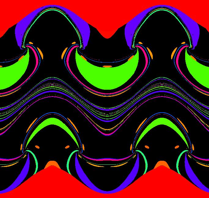
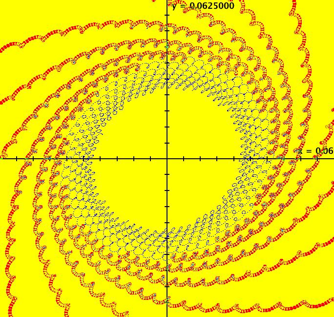
View/Sys/Gal: EMap "PendulumExs: (5.1j) (y,-k*sin(x)-c*y+d*sin(t)), EMapCT3, infinite monkeys" in "PhysicsExs." This is the EMap view of the driven pendulum. The Ode solution curves are also somewhat interesting in the 3D view. This iteration is defined by: x <- y, y <- -k*sin(x)-c*y+d*sin(t). Parameters are: k = 2.50; c = 1.30; d = -.35; Image 1: EMap view, one monkey. Image 2: Ode view. --> In the EMap view, zoom out to see the infinite monkey faces. Image 3: EMap view, zoomed out, infinite monkeys. --> Try various color tables.
|
|
|
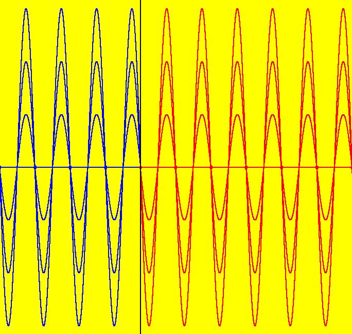
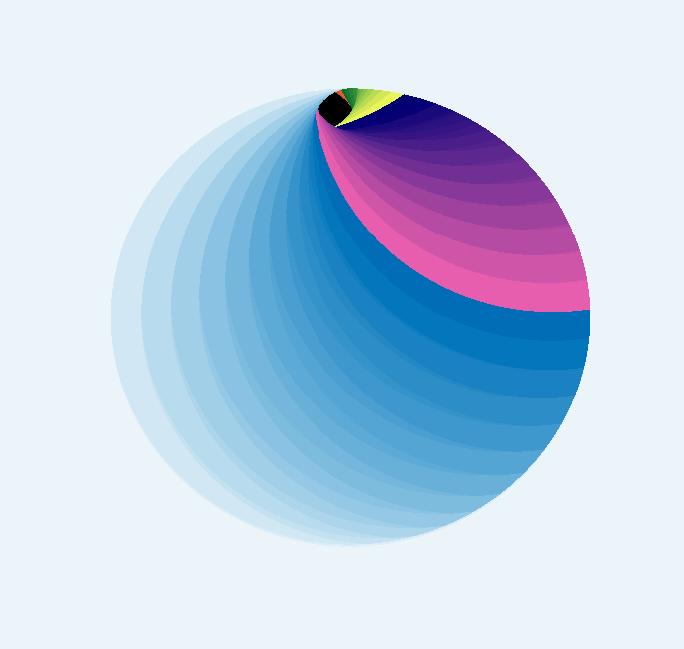
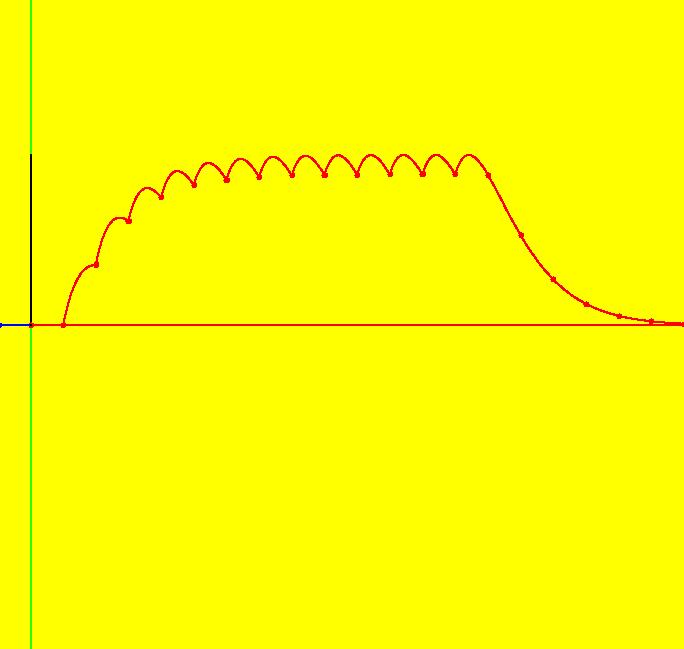
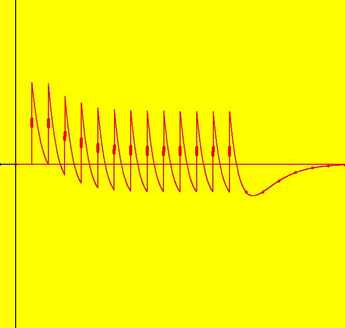
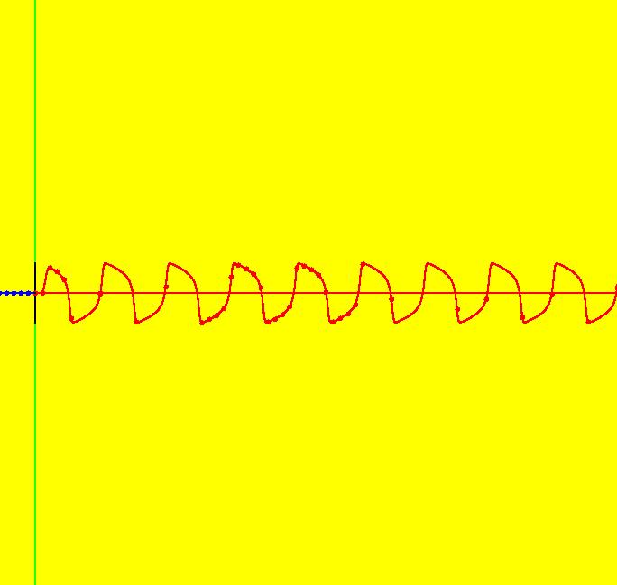
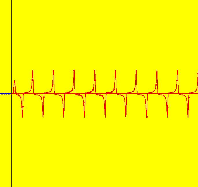
View/Sys/Gal: Ode "PendulumExs: (6.0) Clint Sprott's happiness model" in "PhysicsExs." The "Fig. n" references at the end of the system (6.1) through (6.6) system names correspond to figures in the "Happiness" model paper by Clint Sprott, 2005. Sprott's paper is based on a novel reinterpretation of the damped driven linear harmonic oscillator model written as: R''+ β*R'+R = F(t) (2) where the damping term dR/dt is "happiness" and the driving function, F(t), corresponds to "happy" or "sad" events encountered during life. In OdeFactory notation the 2nd order ode given by equation (2), written in normal form, is: y'' = -b*y'-y+F in the (x,y,y') coordinate system. Using parameters: b=2; a=1; c=1; d=1; an example of F(t) is: F=a*pulse(t-1)+c*pulse(t-2)+d*pulse(t-3) NOTE: User defined functions in OdeFactory must always be defined in (t,x,y,z,w) coordinates. The OdeFactory pulse function (also called the spike function) is a rectangle of width .02, height 50 and area = 1 sitting at the origin. Positive values for parameters a, c and d represent "happy" events. In OdeFactory, the 1st order 2D system corresponding to (2) is: dx/dt = y, dy/dt = -b*y-x+F in the (t,x,y) coordinate system. The notational change is: R(t) -> x(t), H(t) = dR/dt -> dx/dt = y(t). y(t) = subjective (not measurable, inner) happiness a person feels x(t) = objective? (measurable?, outer) happiness as seen by others Note that x(t) = ∫ y(t)dt but since y(t) is subjective then so is x(t). Consequently you cannot verify the "happiness model" by experiment. If instead you consider the system to be a model for a pulsed damped simple harmonic oscillator, where x(t) is position and y(t) is velocity then x(t) and y(t) are measurable and you could verify the model. Image 1: 3D/(t,x) view, outer happiness vs t. Image 2: 3D/(t,y) view, inner happiness vs t.
|
|
|
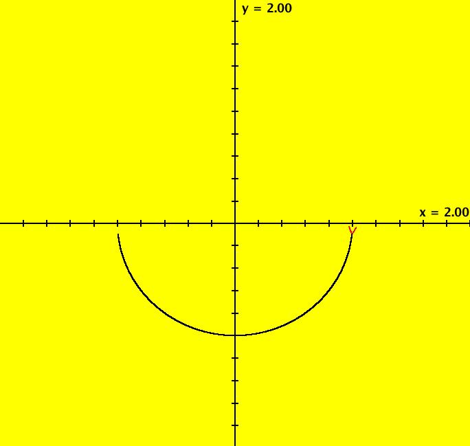
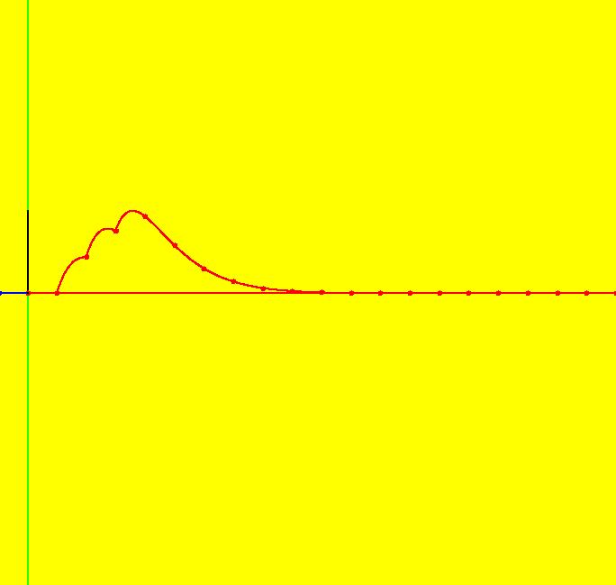
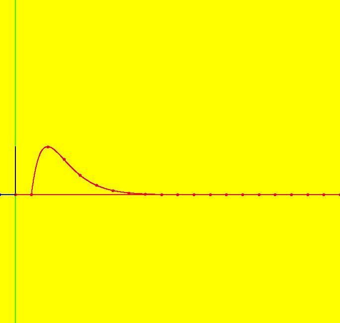
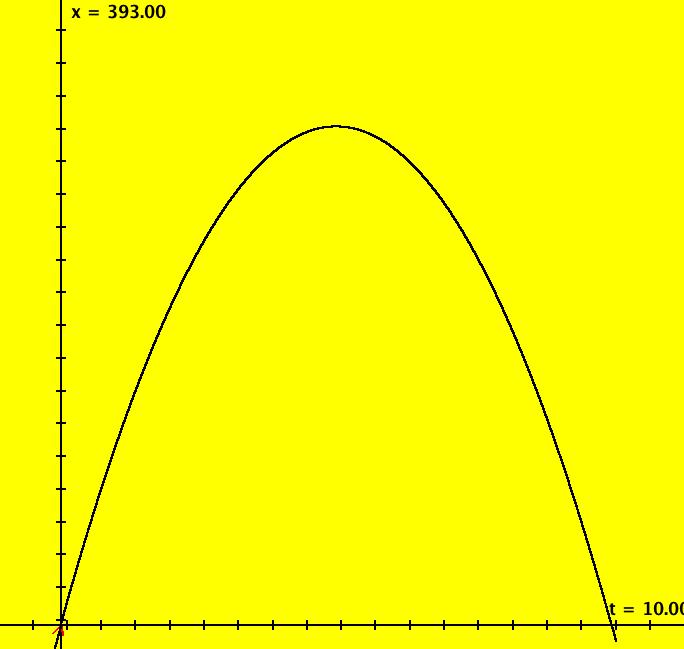
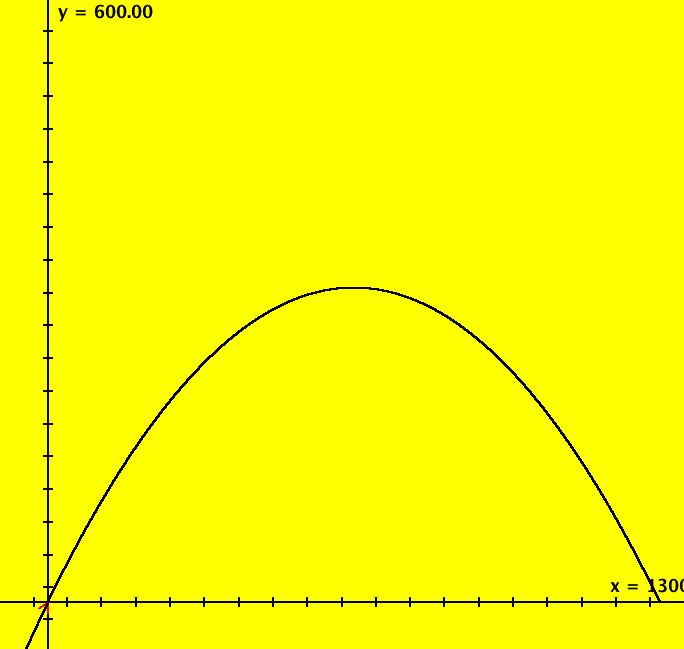
View/Sys/Gal: Ode "PendulumExs: (6.1) winning the lottery, Fig. 2" in "PhysicsExs." This system of odes is defined by the equations: dx/dt = y, dy/dt = -b*y-x+F in the (t,x,y) coordinate system. The 1st order 2D system corresponds to the 2nd order ode: y'' = -b*y'-y+F in the (x,y,y') coordinate system. Parameters are: b=2 Functions are: F=pulse(t-1). In this case F represents a one-time happy event. Image 1: Ode (x,y) view, the projection of the trajectory onto the x axis (friends view) is positive then zero, the projection onto the y axis (winner's view) is positive then negative then zero. Setting hMax = 20 ... Image 2: Ode 3D/(t,x) view, the winner's friends view of the winner's happiness is all positive. Image 3: One 3D/(t,y) view, winner's is happy for a while, not happy for a while, then returns to equilibrium.
|
|
|
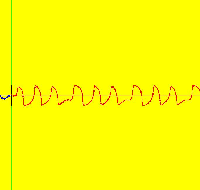
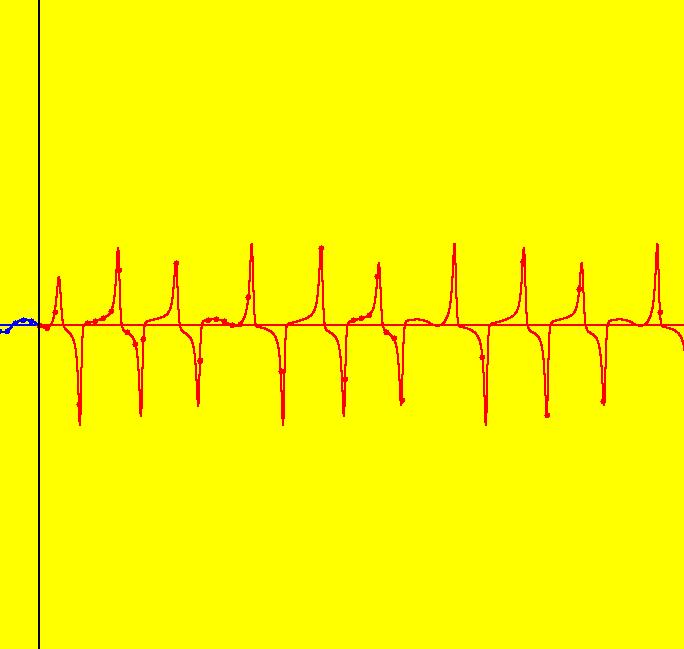
View/Sys/Gal: Ode "PendulumExs: (6.2) drug or other addiction, Fig. 3" in "PhysicsExs." This system of odes is defined by the equations: dx/dt = y, dy/dt = -2*y-x +pulse(t-1)+pulse(t-2)+pulse(t-3) +pulse(t-4)+pulse(t-5)+pulse(t-6) +pulse(t-7)+pulse(t-8)+pulse(t-9) +pulse(t-10)+pulse(t-11)+pulse(t-12) +pulse(t-13) in the (t,x,y) coordinate system. pulse(x) = (x<-eps||x>eps) ? 0 : 1/(2*eps) w/eps = 0.01. Image 1: Ode 3D/(t,x) view: "drug dose" vs time. Image 2: Ode 3D/(t,y) view: "happiness" vs time.
|
|
|
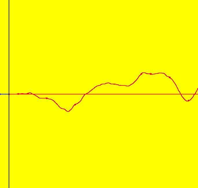
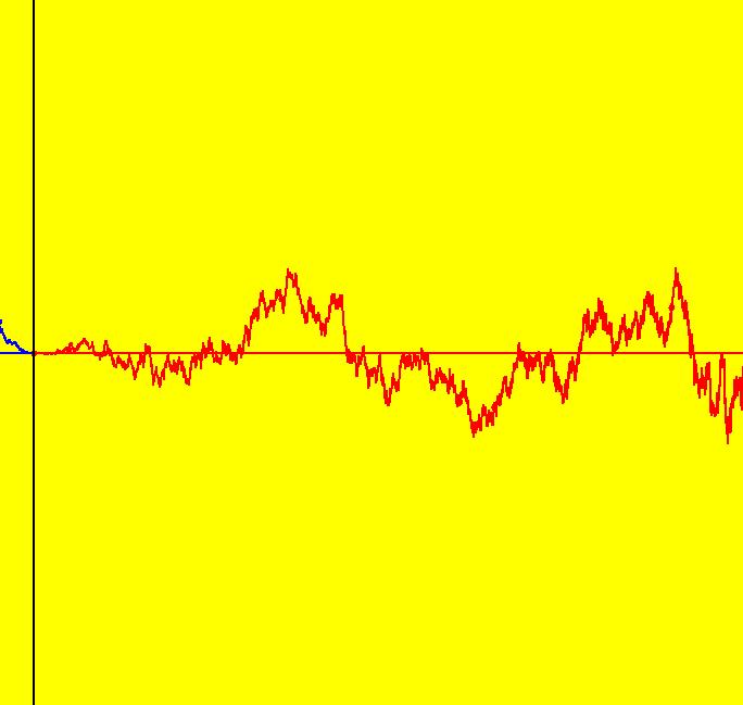
View/Sys/Gal: Ode "PendulumExs: (6.3) real life, Fig. 4" in "PhysicsExs." This system of odes is defined by the equations: dx/dt = y, dy/dt = -2*y-x+a*t*random(-5,5) in the (t,x,y) coordinate system. The 1st order 2D system corresponds to the 2nd order ode: y'' = -2*y'-y+a*x*random(-5,5) in the (x,y,y') coordinate system. Parameters are: a = .430; Image 1: Ode 3D/(t,x) view, "random happy/sad events happen" vs time. Image 2: Ode 3D/(t,y) view, "random happiness" vs time.
|
|
|
View/Sys/Gal: Ode "PendulumExs: (6.4) bipolar disorder, Fig. 5" in "PhysicsExs." This is a nonlinear variation of the "pendulum" system where the nonlinearity is introduced in the damping term: a*(1-x^2)*y. This system of odes is defined by the equations: dx/dt = y, dy/dt = a*(1-x^2)*y-x+b*pulse(t-1) in the (t,x,y) coordinate system. The 1st order 2D system corresponds to the 2nd order ode: y'' = a*(1-y^2)*y'-y+b*pulse(x-1) in the (x,y,y') coordinate system. Parameters are: a = 3.000; b = 1.000; Image 1: Ode 3D/(t,x) view. Image 2: Ode 3D/(t,y) view.
|
|
|
View/Sys/Gal: Ode "PendulumExs: (6.5) chaotic behavior, Fig. 6" in "PhysicsExs." This system is system (6.4) with a periodic driving function used in place of the pulse(t-1) function. This system of odes is defined by the equations: dx/dt = y, dy/dt = a*(1-x^2)*y-x+sin(t)-b in the (t,x,y) coordinate system. The 1st order 2D system corresponds to the 2nd order ode: y'' = a*(1-y^2)*y'-y+sin(x)-b in the (x,y,y') coordinate system. Parameters are: a = 2.900; b = .330; Image 1: Ode 3D/(t,x) view. Image 2: Ode 3D/(t,y) view.
|
|
|
View/Sys/Gal: Ode "PendulumExs: (6.6) anticipation, Fig. 7" in "PhysicsExs." This is an extension of the pendulum system to a higher dimensional system. This system of odes is defined by the equations: dx/dt = y, dy/dt = z, dz/dt = -a*z-b*(1-x^2)*y-x. Parameters are: a = .5; b = -5.6; ICs: p(0.000000) = (0.929889,0.436364,0.000000) Image 1: This is a strange attractor in the z = 0 plane.
|
|
An OdeFactory Slide Show Click on a slide to zoom in. Click "video" to see a video. |
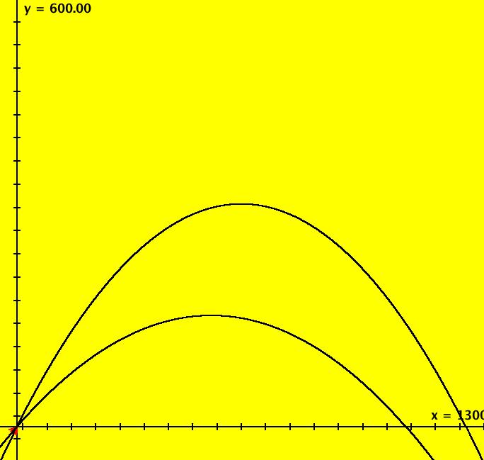
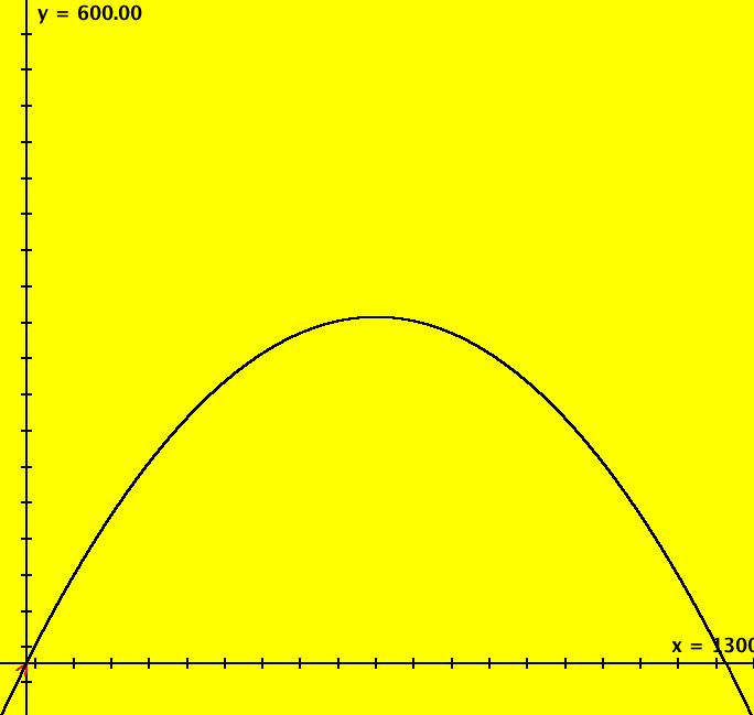
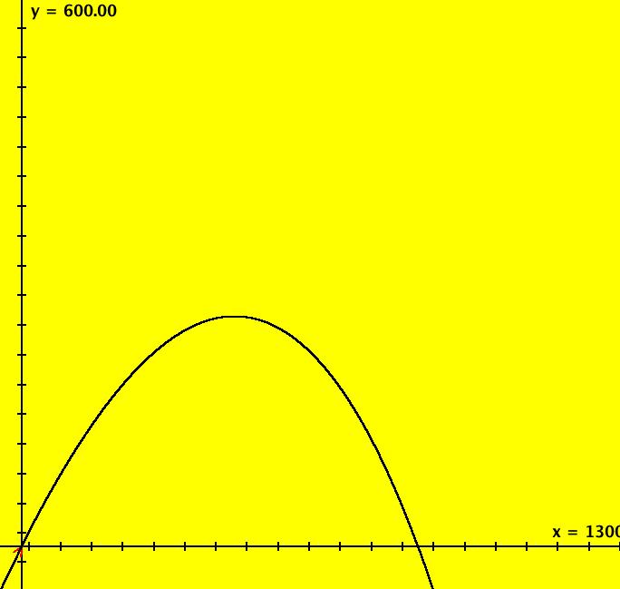
View/Sys/Gal: Ode "ProjectileMotion: Overview" in "PhysicsExs." Projectile Motion The systems in this section model the motion of a projectile moving in two physical dimensions, x and y, with two velocity components dx/dt and dy/dt and with no wind. Depending on special cases, and how the projectile motion is modeled, the number of odes may be 1, 2, 3 or 4. If wind were added OdeFactory could not be used to model the system since 6 odes would be needed. The first 5 systems assume there is no air resistance (drag force) while the last system models an arrow in flight with drag proportional to v^2*area. PDim: physical dimension of the motion MDim: math dimension of the model vars: number of state variables params: number of parameters (g is a constant) auton: yes means autonomous
|