Click on an image to go directly to a system or scroll to see all of the systems in this gallery.
 |
 |
 |
 |
 |
 |
 |
 |
 |
 |
 |
 |
 |
 |
 |
 |
 |
 |
 |
 |
 |
 |
 |
 |
 |
 |
 |
 |
 |
 |
 |
 |
 |
 |
 |
 |
 |
 |
|
 |
 |
 |
 |
|
 |
 |
 |
 |
 |
 |
 |
 |
 |
 |
|
|
|
 |
 |
 |
 |
 |
 |
 |
 |
 |
 |
 |
 |
 |
 |
 |
 |
 |
 |
 |
 |
 |
 |
 |
 |
| OdeFactory Images and Annotations | |||||||||||||||||||||||||||||||||||||||||||||||||||||||||||||||||||||||||||||||||||||||||||||||||||||||||||||||||||||||||||||||||||||||||||||||||||||||||||||||||||||||||||||||||||||||||||||||||||||||||||||||||||||||||
|
An OdeFactory Slide Show Click on a slide to zoom in. Click "video" to see a video. |
View/Sys/Gal: Ode " Dynamical System Topics" in "DynamicalSysExs." OdeFactory is an integrated development environment for creating and studying dynamical systems defined by vector fields of low dimension (<=4). The "dynamics" of the systems can be animated in OdeFactory. The examples in this gallery illustrate the relationship between: (a) time, state space, parameter space and dimension, (b) continuous time and discrete time, (c) analytically and geometrically defined features of dynamical systems. The following topics are covered. phase space, extended phase space, param space: * phase space or state space: (x,y,z,w) * dim of phase space, degrees of freedom * extended phase space: (x,y,z,w,t) * parameter space: (a, b, ...) vector fields: * defining a vector field * viewing a vector field * motion defined by a vector field * nullclines for 2D systems * complex numbers as 2D vector fields * slope fields for 1D systems creating/deleting/editing: * trajectories (Odes) and * orbits (Maps) using auto-generated parameter controllers
animation of: * regions of phase space * trajectories, orbits * orbits in prisoner sets in EMaps * strange attractors finding fixed points: * graphically using OdeFactory * analytically using WA * fixed points at ∞ in R2+ finding 2D separatrix systems finding cycles and approximate periods: * in Odes and IMaps * in (x,y), in the 3D/(t,x) view finding strange attractors: * in Odes and IMaps using the Ode/IMap/EMap button: * continuous vs discrete time * a system in different "views" dimensions and promotions: * time -> state variable * nonauton -> auton system * parameter -> state variable * 1D sys w/1-param -> a 2D bifurcation diagram * 2D sys w/2-params -> a 4D bifurcation diagram defining a system w/specific features: * Hamiltonian systems * quasiHamiltonian systems * algebraically generated flows (AGFs) fractals: * in phase space and parameter space * Julia sets and Mandelbrot sets * z <- z^2+c as an AGF exporting: * images, web pages, galleries importing: * systems, galleries The context for the following tables includes nonautonomous, nonsmooth and discrete systems.
@: no transients #: includes IMaps and EMaps -: means does not apply +: a slope field display Notice that the 2D column contains all yeses. Historically the qualitative features of 2D systems have been studied the most. This is because they are the easiest to visualize graphically.
|
|
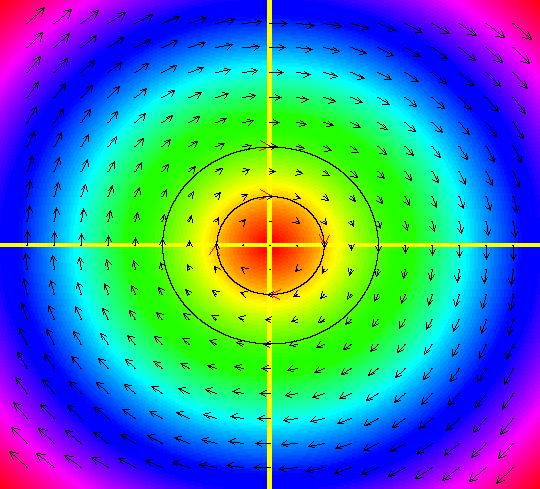
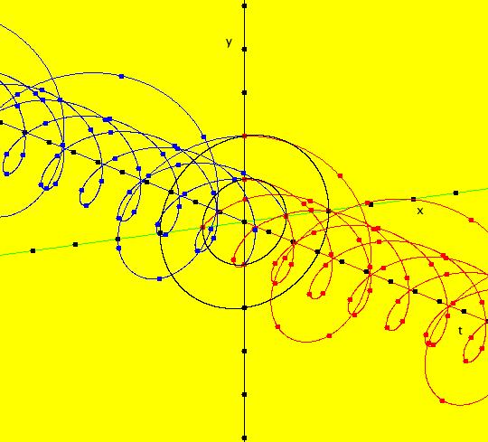
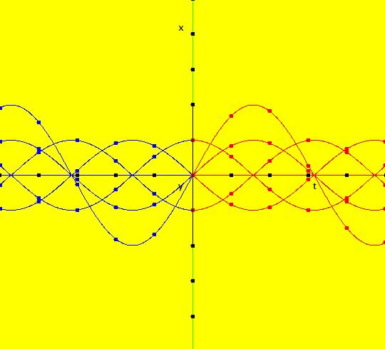
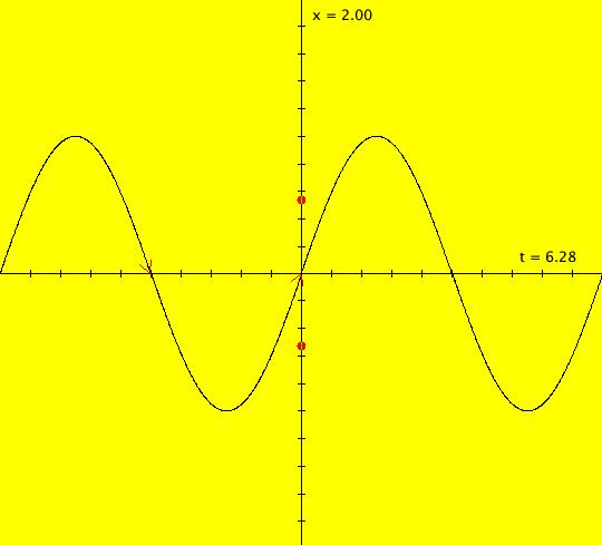
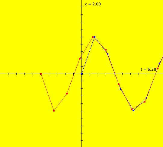
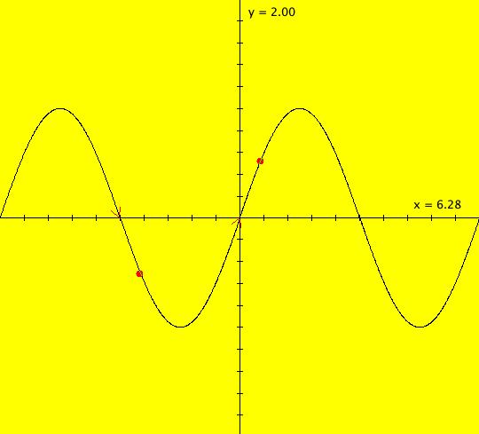
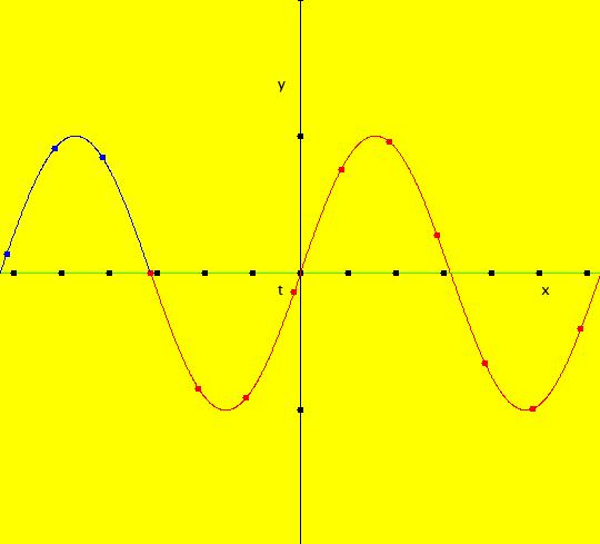
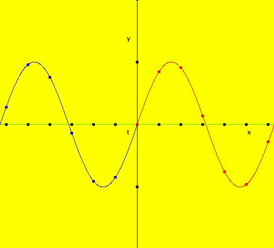
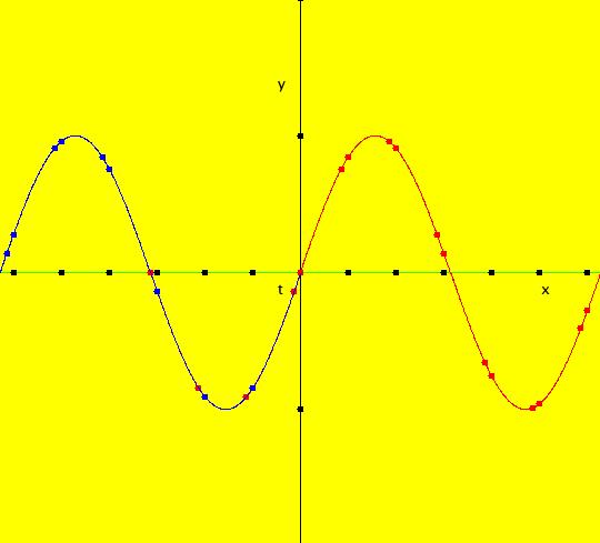
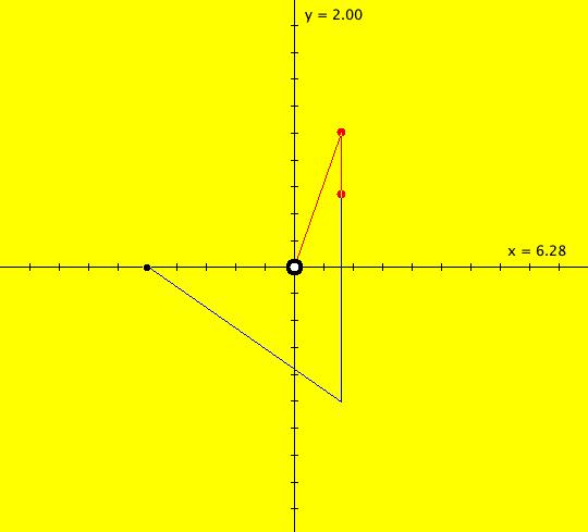
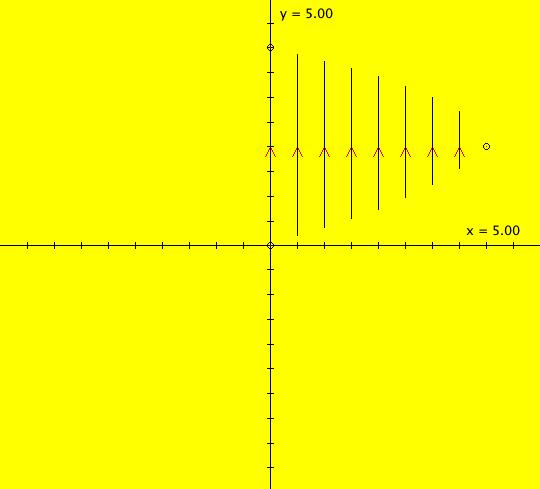
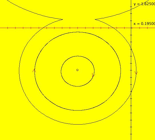
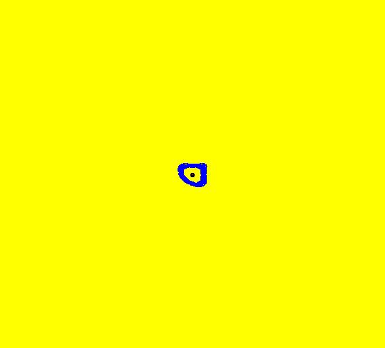
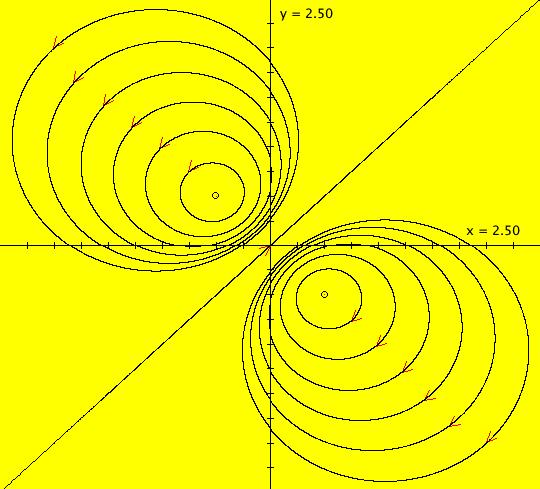
View/Sys/Gal: Ode "( 1a) 2D circles: (y,-k*x/m), k=1; m=1" in "DynamicalSysExs." This system of odes is defined by the equations: dx/dt = y, dy/dt = -k*x/m in the (t,x,y) coordinate system. The 1st order 2D system corresponds to the 2nd order ode in normal form: y'' = -k*y/m in the (x,y,y') coordinate system. Parameters are: k=1; m=1 The system can be entered in OdeFactory as a 2D 1st order system of odes or as a 2nd order ode in normal form. The dynamical system models the simple harmonic oscillator - a mass on a spring or a pendulum with small amplitude. See system "(1.0) (y,-x) SHO" in gallery PendulumExs for a more complete discussion of the simple harmonic oscillator. In the ode view, for k = m = 1 we get circles. In general, the trajectories are ellipses. The (x,y) plane is the phase space. The extended phase space is the 3D space (t,x,y), where the +t axis is out of the screen directly into your eye. NOTE: the default value of t0 is 0, so the "(x,y)" plane is generally the (0,x,y) plane in 3D. If you want to use a different of value of t0, you need to use shift-L-click to set t0 before you enter any ICs for a system. (1) View the colored vector field in the phase space. Note the nullclines. Zoom in on the fixed point at the origin where the nullclines cross. Image 1: The phase space with colored vector field and nullclines. (2) In the 3D/(t,x,y) view, you can see the circles in the (x,y) plane coming toward you. The trajectories you see in the (x,y) plane are the projections of the solution curves in the extended phase space, (t,x,y), onto the (x,y) plane. The black curves are the projections of the solution curves onto the phase space. The red part of a solution curve is the +t part and the blue part is the -t part. The dots on the solution curves are one t unit apart. The solution curves show the future, and past, history of the motion - but not the motion itself. --------------------------------------------- Note that a single trajectory curve in the 2D phase space corresponds to an infinite family of solution curves in the 3D extended phase space and the family of solution curves lies on a 2D surface and if the system is autonomous, it is perpendicular to the phase space. The members of the family of solution curves all have different (x0,y0) starting points, or ICs, on the trajectory. --------------------------------------------- In the 3D/(t,x) view, count red dots on an x(t) curve, and note that the period looks like it might be 2 π. If you select "Show Approximate Period" on the Settings menu you get a computed approximate period for the last trajectory drawn of 6.270, i.e. about 2 π. Image 2: The extended phase space, in the 3D/(t,x,y) view. (3) Start a Flow with (dots,speed,secs) = (0,.90,20) and note that the 5 dots starting at the arrowheads orbit the origin at the same angular rate. This demonstrates the fact that the period is constant. Image 3: The extended phase space, in the 3D/(t,x) view. (4) Adjust k and m. Physically k and m are significant. Mathematically only the ratio k/m is significant.
|
|
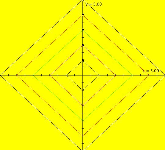
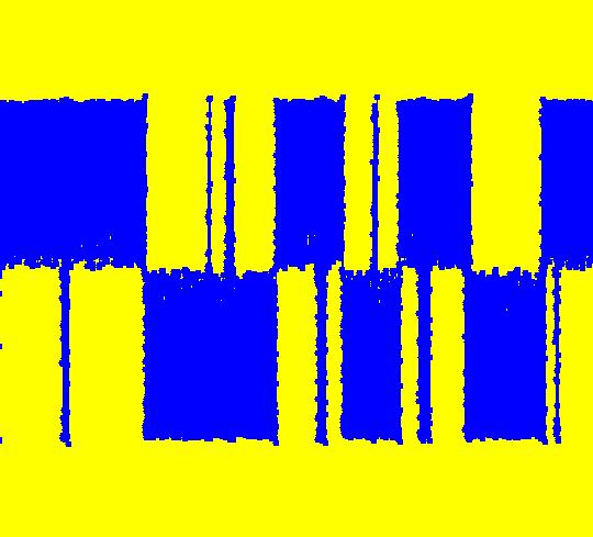
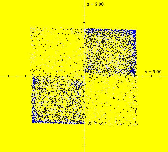
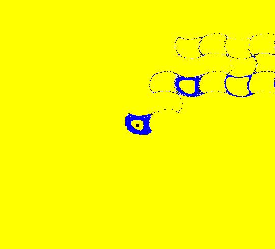
View/Sys/Gal: EMap "( 1b) 2D squares from ( 1a), IMap1100" in "DynamicalSysExs." This iteration is defined by: x <- y, y <- -k*x/m. Parameters are: k=1; m=1 This is the IMap view of system ( 1). (1) Start a Flow. As orbits are defined, they are colored cyclically: blue, red, green, magenta, black, blue. Note that only the last orbit defined, in this case, the black inner orbit with seed at (0,1), is animated. If you delete the black orbit, the new "last" orbit will be animated. Image 1: The phase space. (2) When k = m = 1, all orbits are squares with period 4. To see that the period is 4, note that: p0 = (x,y) -> p1 = (y,-x) -> p2 = (-x,-y) -> p3 = (-y,x) -> (x,y) = p0. Image 2: After setting hMax = 50, the extended phase space, 3D/(t,x) view. To prove that the orbits are square, show that for any orbit: (a) p0, p1, p2, p3 are all the same distance from the origin p = (0,0), sqrt(x^2+y^2) and (b) that the distance between consecutive points is sqrt(2*(x^2+y^2)). All points on an orbit stay within a circle of radius sqrt(x^2+y^2) so in the IMap view, all orbits starting inside or on the circle of radius sqrt(50) stay in or on the circle and all orbits starting outside of the circle stay outside of the circle. In the EMap view the black circle of radius sqrt(5) is the "prisoner" set. Image 3: Zoomed out EMapCT0 view, last orbit showing. (3) Start an off-axis orbit and try Flow again. (4) Adjust k and m. All orbits for parameter values not equal to 1 are spirals (in or out).
|
|
View/Sys/Gal: EMap "( 2) 2D mapping of a region in the phase space" in "DynamicalSysExs." The motion of a dynamical system occurs in the phase space. Since the computer screen is a 2D space, it is easiest to view the motion for 2D systems which have a 2D phase space. Consider the system, dx/dt = x+y, dy/dt = -a*x with a = 2. Image 1: The vector field for the system. Geometrically, you can think of an ode as defining a continuous mapping of a region, R(0), in phase space into another region, R(t), in phase space, or, as a deformation of the phase space. (1) To see how the mapping works, you need to draw a region to be mapped before you start an animation: (a) select "Hide 2D Ode Trajectories" (b) drag to draw a region free-hand (c) click Flow and start the animation.
Step (a) is not required but it can be used to create better looking animations. You can run the animation for an Ode in either the +t (red dots) or the -t (blue dots) direction. You can animate whatever curve you draw. Image 2: Animation of a hand-drawn region. (2) You can also animate a selection square as follows: (a) ctrl-drag to create a selection square (b) click "Flow" and start the animation. Image 3: Animation of a selection square. (3) You can animate hand-drawn regions and a selection square at the same time.` (4) You can animate the vector field itself by varying the parameter "a." Turn on the vector field then open the parameter controller and adjust "a." This simple linear system can also produce fractals. Go to the EMap view and select color table 9. Zoom all the way in. Image 4: The EMapCT9 view shows a fractal. For a = 1, the IMap has period 6.
|
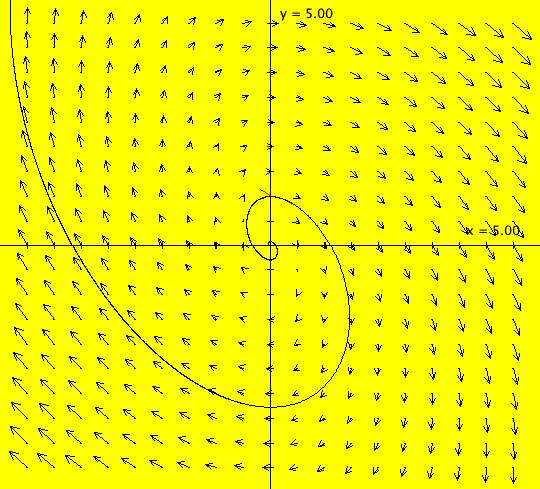
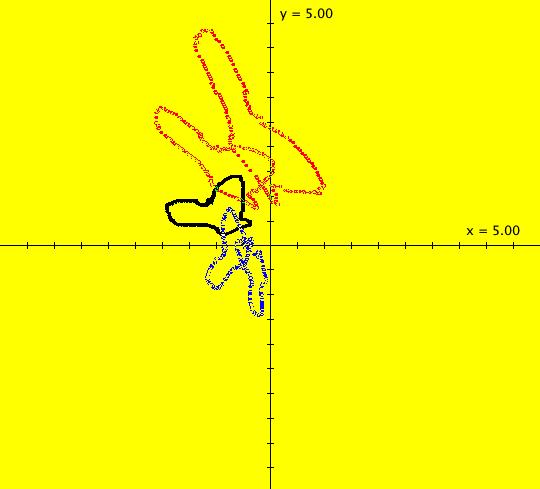
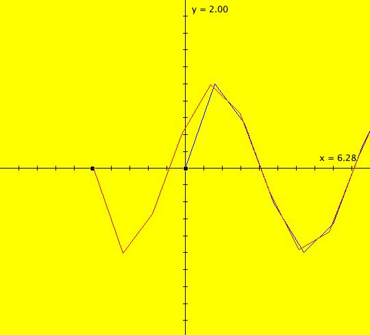
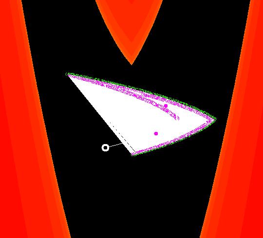
| View/Sys/Gal: EMap "( 3) 2D finding limit cycles & periods" in "DynamicalSysExs." This system of odes is defined by the equations: dx/dt = y, dy/dt = a*x+cos(x)*y. Parameters are: a = -2 There are an infinite number of limit cycles for a < 0. This result was proven in 1980 by Zhang Zhi-fen. The system is also discussed on p. 311 of Hubbard and West, "Differential Equations: A Dynamical Systems Approach, Higher-Dimensional Systems." To find an approximate limit cycle start a trajectory, click on its arrowhead, and extend it in +t and -t. Start new trajectories at the +t and -t ends of the first trajectory, then delete the first trajectory. Repeat the process to find additional limit cycles. For the limit cycles (outer to inner) in the image:
Image 1: Five approximately periodic trajectories. Image 2: Zoomed-in view of outer trajectory near the starting point. A Monte Carlo method can also be used to find the limit cycles for this system. Start a flow with: (trajs, speed, sec) = (150,.9,180). Click "Start Flow" three times in rapid succession to generate 450 random dots. Do this with +t and then with -t. The red dots show the +t ω-limit sets and the blue dots show the -t α-limit sets. Image 3: Monte Carlo method for 450 random red dots in +t and 450 random blue dots in -t. Values of a = -1 and 1.8 give interesting EMaps when you zoom in. Image 4: The EMap view zoomed in with CT 2.
|
|
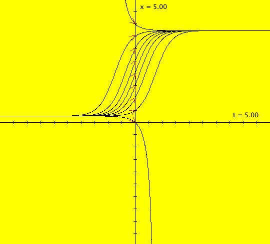
View/Sys/Gal: IMap "( 4a) 1D nonautonomous motion in the phase space" in "DynamicalSysExs." This ode is defined by the equation: dx/dt = cos(t). The system is called nonautonomous because of the explicit time dependence of the vector field, i.e. the cos(t). The x axis is the phase space. The vector field, which is defined in the phase space, is not shown for 1D systems because it provides little visually useful information in the 1D space. Furthermore, vector fields are not shown for any nonautonomous systems since they are not constant in time. The 2D (t,x) plane is the extended phase space which contains the solution curves. Tangents to the solution curves do provide useful visual information so they can be shown in OdeFactory using the "S On/Off" button. The sin(t) curve is a single solution curve. Two trajectories have been started at: IC1 = (t1,x1) = (- π,0) and IC2 = (t2,x2) = (0,0). --------------------------------------------- Note that for 1D systems t0 is not defaulted to 0 as it generally is for systems of higher dimensions. In this example t1 ≠ t2 while x1 = x2. --------------------------------------------- The general solution to the ode is x(t) = x(t0)+sin(t). The ICs give x(- π) = x(0) = 0 so both solution curves, in the extended phase space, i.e. the (t,x) plane, coincide and are just x(t) = sin(t). The projection of a solution curve onto the phase space is called a trajectory. The "motion" defined by the system is on the trajectory in the phase space.
The extended phase space shows the future, and past, history of the motion, but not the motion itself. (1) To see the motion associated with the system, start a "Flow." Vary the Flow parameters as needed. The red dot moving down shows the motion on the trajectory associated with IC1 and the red dot moving up shows the motion on the trajectory associated with IC2. The two trajectories on the x-axis happen to lie on top of each other. Note: In the 1D Ode view, if a solution curve exits the graphics area, the corresponding dot on the x-axis vanishes. When/if the solution curve reenters the graphics area the corresponding dot reappears. To see this happen, shift the sine curve up so the peaks are out of the view and start a Flow. In the Ode view, all solution curves are x-translates of the sine curve. The left-most solution curve starts at (t,x) = (- π,0) and the solution to the right starts at (t,x) = (0,0). Image 1: Start of a Flow. The red dot initially moving down on the -x axis is on the trajectory of the solution starting at (- π,0) while the red dot imitially moving up on the +x axis is on the trajectory of the solution starting at (0,0). In the IMap view the sine curve through (0,0) is an attractor for all orbits. Image 2: IMap view of the sine curve attractor. The red IMap orbit corresponds to the Ode solution curve starting at (- π,0) and the blue IMap orbit corresponds to the Ode solution curve starting at (0,0).
|
|
View/Sys/Gal: IMap "( 4b) 2D autonomous version of the Ode view of ( 4a)" in "DynamicalSysExs." This system of odes is defined by the equations: dx/dt = 1, dy/dt = cos(x). This is the 2D autonomous version of the 1D nonautonomous system ( 4a) dx/dt = cos(t). System ( 4a) is defined in the (t,x) coordinate system and ( 4b) is defined in the (x,y) coordinate system. See OdeFactory gallery NonAutonToAutonExs for a general discussion of how to convert a nonautonomous system to the corresponding autonomous system. To get from ( 4a) to ( 4b), in system ( 4a) replace x by y and t by x so ( 4a) becomes ( 4a) dy/dx = cos(x). Then write dy/dx = (dy/dt)/(dx/dt) = cos(x)/1 so ( 4b) is dx/dt = 1, dy/dt = cos(x). The phase space for ( 4b) is the (x,y) plane and the extended phase space for ( 4b) is R3, (t,x,y). The +t axis is out of the screen directly into your eye. The ICs for ( 4a) correspond to IC1 = (0,x0,y0) = (0,- π,0) and IC2 = (0,0,0) in system ( 4b). (1) Try a Flow animation with parameters (0,.9,60). (2) We are viewing ( 4b) in the phase space (the trajectories). The 3D/(t,x,y) view shows ( 4b) in the extended phase space view (the solution curves). 3D/(t,y) shows the y-component of the solution curves, y(t). Image 1: Start of a Flow in the (x,y) phase space. Here we are viewing the trajectories of the 2D system in the (x,y) phase space and the flow, or motion, is shown by the red dots on the trajectories. Image 2: The 3D/(x,y) Ode view of the left most trajectory starting at (t,x,y) = (t.- π,0). Image 3: The 3D/(x,y) Ode view of the other trajectory starting at (t,x,y) = (t.0,0).. Image 4: The 3D/(x,y) Ode view of both trajectories. Image 5: The 3D/(t,x,y) Ode view of both trajectories. The IMap (x,y) -> (1,cos(x)) -> (1,cos(1)) has a fixed point at (1,.5403023). Image 6: The IMap fixed point in the IMap view. The red dot at (1,.5403023) is the fixed point.
|
|
View/Sys/Gal: IMap "( 4c) 2D autonomous version of the IMap1000 view of ( 4a)" in "DynamicalSysExs." This iteration is defined by: x <- 1+x, y <- cos(x). To get the IMap version of ( 4a) you need to use: x <- 1+x rather than x <- 1. Note that the Ode version of ( 4c) is not the same as the Ode version of ( 4a). Image 1: IMap view of sine curve attractor. All orbits have period 1.
|
|
View/Sys/Gal: IMap "( 5) 2D periodic orbits in the hopalong, IMap1100" in "DynamicalSysExs." This iteration is defined by: x <- y-cos(x), y <- a-x. Parameters are: a=-2.3 "Flow" animation is enabled for 2D IMaps but only for the last orbit that has been defined. If all orbits were animated it would be too difficult to follow the animation. The animation follows the orbit when it is out of the view so if the orbit returns to the view the dots will return. This enables you to watch for approximate periodic orbits. (1) Start a "Flow" animation at Max speed for 120 sec. Image 1: 20 seconds into the animation. (2) Click on the seed to see how many iteration steps were done while drawing the lines. (3) Extend the orbit in +t. In the current zoomed-in view we see that the orbit is not exactly periodic. If you zoom out 9 times it looks more like the orbit has approximate period 4. Try the animation again. Image 2: Image 1 zoomed out. Image 1 is of the upper right hand corner of image 2. OdeFactory give period = 2272 for the orbit. (4) Find a periodic orbit with period 4. Answer: (x,y) = (2.339023,1.644162). Google "Barry Martin hopalong map" for more information on this map. See OdeFactory gallery MapExs for variations of the map.
|
|
View/Sys/Gal: IMap "( 6a) 1D logistic IMap0100" in "DynamicalSysExs." This iteration is defined by: x <- r*x*(1-x). Parameters are: r=3.5 Reference: logistic map. "Flow" animation is not enabled for 1D systems in the IMap view because it would not provide any useful new information. The time series already shows the history of the motion. Generally we want to see the pattern of the iteration values as r changes. The best way to do this is to simply vary r by using the +r and -r buttons in the "Adj Ctrl Params" window. Image 1: A period 4 cycle. (1) Try adjusting r. (2) See the Ode view.
|
|
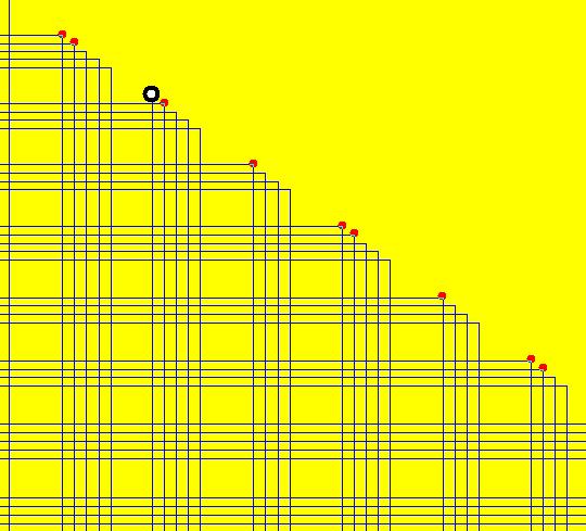
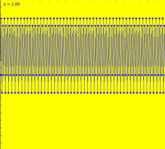
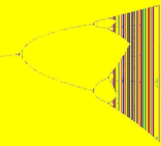
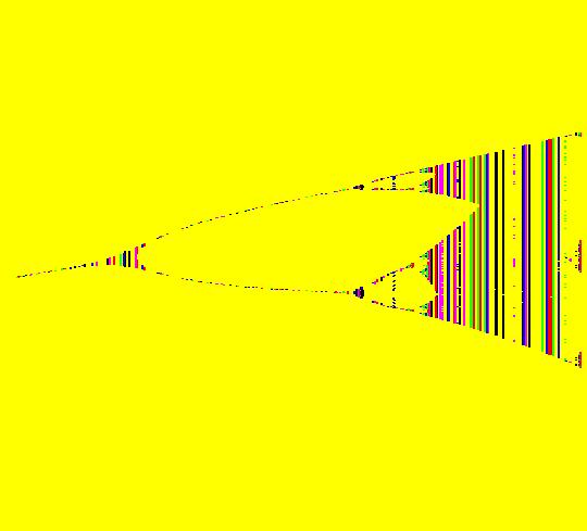
View/Sys/Gal: IMap "( 6b) 2D logistic map's bifurcation diagram, IMap0111" in "DynamicalSysExs." This iteration is defined by: x <- x, y <- x*y*(1-y). This 2D system is being used to generate the bifurcation diagram of the 1D logistic map x <- r*x*(1-x), where r is the bifurcation parameter. The bifurcation diagram is also called a Feigenbaum diagram. NOTE: the "busy" cursor is shown in the graphics window while the image, which has 434 seeds, is being rendered. It takes a lot of seeds (x values for this 2D system correspond to r values for the corresponding 1D logistic map) to generate a bifurcation diagram so you may need to wait a bit for the image to be completed. In OdeFactory, if you promote the parameter of a 1D map to a constant state variable in a 2D IMap, the 2D map becomes the bifurcation diagram for the 1D map. The 2D system is constructed by first replacing x by y in the 1D logistic map and rewriting the iteration as y <- r*y*(1-y). Next replace the bifurcation parameter r by the "variable" x and write the 2D system as: x <- x, y <- x*y*(1-y). Now x's IC's play the role of different r's in the original 1D map. The IMap view of the 2D system shows the orbits of the 1D system as dots projected onto the vertical lines x = r. See "Nonlinear Dynamics and Chaos," by Steven Strogatz p. 357 fig 10.2.7 for more details concerning the logistic map and it's bifurcation diagram. (1) To generate the bifurcation diagram, start several orbits in the IMap view. Vertical lines with n dots are period-n orbits of the 1D system. Solid vertical lines are chaotic orbits of the 1D system. Image 1: The bifurcation diagram for the logistic map ( 6a). (2) To view an orbit of period 2, clear the IMap view then start an orbit at (3.4,.5). Run a flow animation. You will see red dots accumulating on the line x = 3.4 at about y = .447 and y = .839. Another way to view this orbit is to change hMax to 100 and go to the 3D/(t,y) view to see the time-series for the orbit. In the original image, starting on the left, the open "windows" in the bifurcation diagram show the period-doubling of the periodic orbits. (3) Click in the windows to start a new orbit and note the orbit's period. (4) Find a period-3 orbit and display it in the 1D system ( 9) as follows: (a) The large window on the right looks like it corresponds to a 3-cycle. Click in the window to check this out. Clicking at about (x,y) = (3.831111,0.593939) gives a 3-cycle. (b) Go to the 1D system ( 6a), set r = 3.831111 in the "params:" field, update the system then start an orbit at (t,x) = (0,.5). (5) View the fractal structure of the IMap image as follows: (a) Select a small window, say one of the 8-cycle windows, then zoom in on it. (b) Clear the orbits and create new orbits to regenerate the smaller IMap. Image 2: The top 8-cycle window, at about (x,y) = (3.564,.883), zoomed in. (c) Repeat the process using a 16-cycle window, then a 32-cycle window.
|
|
View/Sys/Gal: Ode "( 6c) 1D fish harvesting (x*(4-x)-k), k=1" in "DynamicalSysExs." This ode is defined by the equation: dx/dt = x*(4-x)-k in the (t,x) coordinate system. Parameters are: k=1 If x is the number of fish (say in thousands) then only x >= 0 is of interest. Image 1: k = 1. ICs (t,x) = (0,1), with k = 1, give: p(100.000000) = (3.732051) p(-100.000000) = (0.267949) which says that
x -> 3.732051 as t -> ∞ and x -> 0.267949 as t -> - ∞. The point (t,x) = (0,3.732051) is a stable fixed point and the point (t,x) = (0,0.267949) is an unstable fixed point. If you follow the horizontal parts of the solution curves back to the x axis you get these two points. As you increase k the fixed points come together and merge into a semi-stable fixed point at (0,2) for k = 4. For k > 4 there are no fixed points.
|
|
View/Sys/Gal: EMap "( 6d) 2D fish harvesting bifurcation diagram" in "DynamicalSysExs." This system of odes is defined by the equations: dx/dt = 0, dy/dt = y*(4-y)-x. The parabola: x = y*(4-y), for x >= 0, is the bifurcation curve for the fish harvesting Ode. Image 1: ICs: (x,y) = (n/2,2) for n = 0, 1, 2, 3, ..., 8 show the outline of the bifurcation parabola. The trajectory with ICs (x,y) = (1,2) corresponds to the (t,x) = (0,2) solution curve shown in system ( 6c). In this system, it goes to y = 3.732051 as t -> ∞ and to y = 0.267949 as t -> - ∞. Image 2: The right edge of the black region of the EMap of this system also shows the outline of the bifurcation parabola. See Gustafson for a discussion of the "fish harvesting" model.
|
|
View/Sys/Gal: Copy of current gallery saved to: "DynamicalSysExs." This 1D iteration is defined by: x <- x^2+a. Parameters are: a = -1.76; Image 1: The seed is at (t,x) = (0,.5) and the period is 3. Notice the transient from t = 0 to about t = 9. Find a 4 cycle and a 2 cycle by varying parameter "a."
|
|
View/Sys/Gal: IMap "( 7b) 2D (x,x+y^2) IMap0011 bifurcation diagram of ( 7a)" in "DynamicalSysExs." This iteration is defined by: x <- x, y <- y^2+x. The period 3 orbit of system ( 7a) is at (x,y) = (-1.76,0). Start a Flow to see where the period 3 orbit is in the bifurcation diagram. Drag in the graphics area to make the period 2 and 4 windows easier to see.
|
|
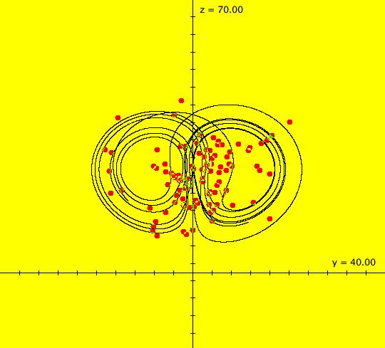
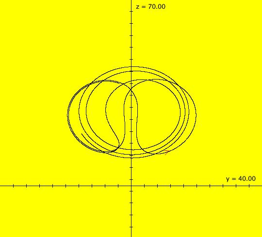
View/Sys/Gal: IMap "( 8a) 2D nonautonomous IMap w/strange attractor" in "DynamicalSysExs." This iteration is defined by: x <- y, y <- -k*sin(x)-c*y+d*sin(t). Parameters are: k = -3.100; c = .030; d = .034; This is system (5.1g) from OdeFactory gallery "PendulumExs." It is an oscillating IMap strange attractor. The attractor consists of the two 3 by 3 square regions in the first and third quadrants. ICs: (t,x,y) = (0,1.759259,-1.434343). 10,000 iterations. Image 1: Result of a Flow animation at max speed for 60 sec. For another view of the oscillation, set hMax = 10000 then go to the 3D/(t,x) view. Image 2: The 3D/(t,x) view. Try adjusting the parameters.
|
|
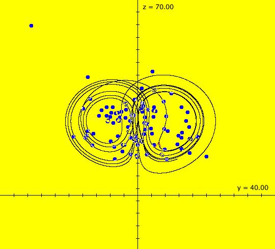
View/Sys/Gal: IMap "( 8b) 3D equivalent autonomous IMap ver of ( 8a)" in "DynamicalSysExs." This iteration is defined by: x <- x+1, y <- z, z <- -k*sin(y)-c*z+d*sin(x). Parameters are: k = -3.100; c = .030; d = .034; ICs: (x,y,z) = (0,1.759259,-1.434343). 10,000 iterations. See gallery "NonAutonToAutonExs" to see how the conversion from system ( 8a) to ( 8b) is done. (1) Start an animation at max speed for 60 sec to see the oscillation.
|
|
View/Sys/Gal: IMap "( 9a) 2D orbit evolution, IMap" in "DynamicalSysExs." This iteration is defined by: x <- y-cos(x%b), y <- a-x. Parameters are: a = -6.500; b = -6.500; Start an orbit at: (x,y) = (0.925926,0.464646) Image 1: 10,000 steps. Zoom out and watch it grow as you extend it 50,000 steps at a time. Image 2: 50,000 more steps. Start a Flow with (0,max,120) and watch how the orbit evolves. Zoom in and investigate how chaotic orbits spread by "leaking" outward.
|
|
View/Sys/Gal: EMap "( 9b) 2D bounded(?) chaotic orbits, IMap0010" in "DynamicalSysExs." This iteration is defined by: x <- y-cos(x%b), y <- a-x. Parameters are: a = -6.500; b = -6.500; Five orbits start at what looks like a single point in the center of the graphics area. If you click on the black dot, you will see that the ICs are: (-5.296296,-1.212121) blue, (-5.296290,-1.212120) red, (-5.296200,-1.212100) green, (-5.296000,-1.212000) magenta, (-5.290000,-1.210000) black. A sixth orbit starts at: (-10.113476,-0.553764) blue. The first five orbits are chaotic i.e. they have approximately the same seeds but they have very different spatial features. Image 1: Five chaotic orbits and one period-4 orbit. If you select "Show Approximate Period" you will see that the sixth orbit has period 4. Zoom out to see the detailed structure of the orbits. Image 2: The period-4 orbit in the EMap view. Extend the orbits. They seem to be bounded, but this may just be an artifact of the floating-point number system being used. If they are bounded, then, in the discrete space defined by the computer's floating-point number system, they are periodic. See "Q&A 63" in the OdeFactory User Guide. Try finding another period-4 orbit.
|
|
View/Sys/Gal: EMap "( 9c) 2D EMapCT10 view of ( 9b)" in "DynamicalSysExs." This iteration is defined by: x <- y-cos(x%b), y <- a-x. Parameters are: a = -6.500; b = -2.000; Try varying the parameters and color tables. Try reproducing this image starting with system ( 9b).
|
|
View/Sys/Gal: IMap "( 9d) 2D a segmented 2.55 milliom iteration orbit, IMap0010" in "DynamicalSysExs." This iteration is defined by: x <- y-cos(x%b), y <- a-x. Parameters are: a = -6.500; b = -6.500; This is one orbit with five segments. There are 2,550,000 iterations. The image is completed when the busy cursor changes to the arrow cursor - be patient. Blue seed: first (x,y) = (-5.296296,-1.212121) last (x,y,t) = (-28.39455092162509, -273.6543580418215, 510000.0) Red seed: first (x,y,t) = (-28.39455092162509, -273.6543580418215, 510000.0) last (x,y,t) = (-37.23378825604409, -256.48469541992336, 510000.0) Green seed: first (x,y,t) = (-37.23378825604409, -256.48469541992336, 510000.0) last (x,y,t) = (-47.689104271024576, -128.46248104749714, 510000.0) Magenta seed: first (x,y,t) = (-47.689104271024576, -128.46248104749714, 510000.0) last (x,y,t) = (-61.164688741400646, -1090.584629954589, 510000.0) Black seed: first (x,y,t) = (-61.164688741400646, -1090.584629954589, 510000.0) last (x,y,t) = (-61.42733285122327, -1090.7800535574386, 510000.0)
|
|
View/Sys/Gal: IMap "( 9e) 2D a single 5.5 million iterations orbit, IMap0010" in "DynamicalSysExs." This iteration is defined by: x <- y-cos(x%b), y <- a-x. Parameters are: a = -6.500; b = -6.500; Wait for the busy cursor to revert to the arrow cursor. This is the blue orbit of ( 9d) extended to 5,510,000 steps. The orbit's last point is at: p = (-81.205813,-1474.841699). The orbit seems to get stuck at p. To investigate what happens at p: * clear the view, * center at p, * zoom in 7X, * start an orbit at p, * center, * extend the orbit 17X.
|
|
View/Sys/Gal: Ode "( 9f) 2D IMap vs Ode views" in "DynamicalSysExs." This iteration is defined by: x <- y-cos(x%b), y <- a-x. Parameters are: a = -6.500; b = -6.500; In the center of the IMap view, seed (x1,y1) = (-5.296296,-1.212121) gives: last (x,y,t) = (-11.344944451412122, 0.39836072440000336, 10000.0) and seed (x2,y2) = (-5.296295999999,-1.212120999999) gives: last (x,y,t) = (-9.097421070595155, -2.021709639122001, 10000.0). Since the two seeds are very close while the final points on the orbits are not, the IMap orbit seems to be chaotic. Image 1: IMap orbits from seeds (x1,y1) and (x2,y2) for 10,000 steps. There is a blue orbit covered by a red orbit. Image 2: Red/blue IMap orbits from seeds (x1,y1) and (x2,y2) extended by 50,000 steps. In the Ode view, using the same two ICs, IC (x1,y1) = (-5.296296,-1.212121) gives: last (x,y,t) = (-6.360418651636713, 1.0367636251781969, 100.00000000001425) and IC (x2,y2) = (-5.296295999999,-1.212120999999) gives: last (x,y,t) = (-6.360418651636712, 1.0367636251782022, 100.00000000001425). so the Ode trajectories are not chaotic. Image 3: The Ode view. In fact the two trajectories go to a limit cycle with period 2 π. A trajectory on the limit cycle starts at (x,y) = (-6.634229,0.958230) and the point (x,y) = (-6.5,1) is a fixed point for the ode. Image 4: The Ode limit cycle and fixed point. Odes trajectories are most often neither chaotic nor periodic while IMap orbits are often a mix of chaotic and periodic orbits. Try varying parameter b.
|
|
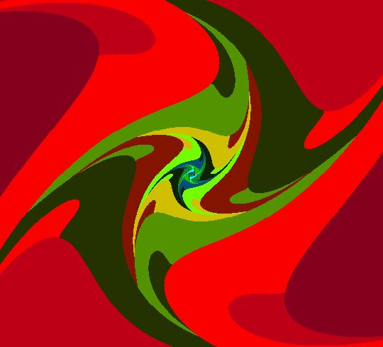
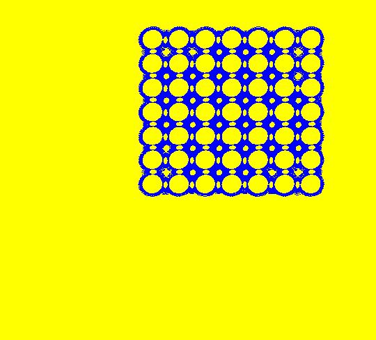
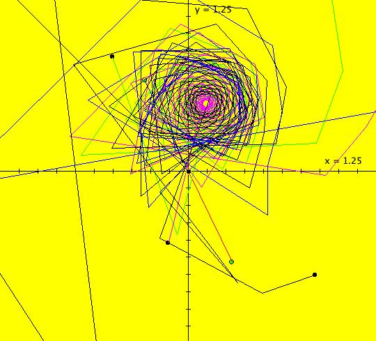
View/Sys/Gal: IMap "( 9g) 2D Oriental Rug Art IMap0111" in "DynamicalSysExs." This iteration is defined by: x <- y-cos(x%b), y <- a-x. Parameters are: a = -.430; b = -.210; This "Art" IMap contains 240 orbits so you may need to wait a bit for the image to be rendered. You can create your own versions of the image by adjusting the parameters and/or by starting different orbits. The color sequence for orbits is: blue, red, green, magenta, black, blue ... As you build an image, if the region you just created is red, and you want it to be black, try starting 3 new orbits in the region to cover up the original red region. The 1st gets you to green, the 2nd to magenta and the 3rd to black.
|
|
View/Sys/Gal: IMap "( 9h) 2D Oriental Rug Art IMap0111" in "DynamicalSysExs." This iteration is defined by: x <- y-cos(x%b), y <- a-x. Parameters are: a = -.430; b = -.190; This "Art" IMap contains 269 orbits so you may need to wait a bit for the image to be rendered. You can create your own versions of the image by adjusting the parameters and/or by starting different orbits. This is a variation of ( 9g). Parameter b was changed from -.210 to -.190 and different seeds were used.
|
|
View/Sys/Gal: IMap "( 9i) 2D Oriental Rug Art IMap0111" in "DynamicalSysExs." This iteration is defined by: x <- y-cos(x%b), y <- a-x. Parameters are: a = -.430; b = -.210; There are 73 orbits in the image. This is just ( 9g) again, zoomed in and with different seeds.
|
|
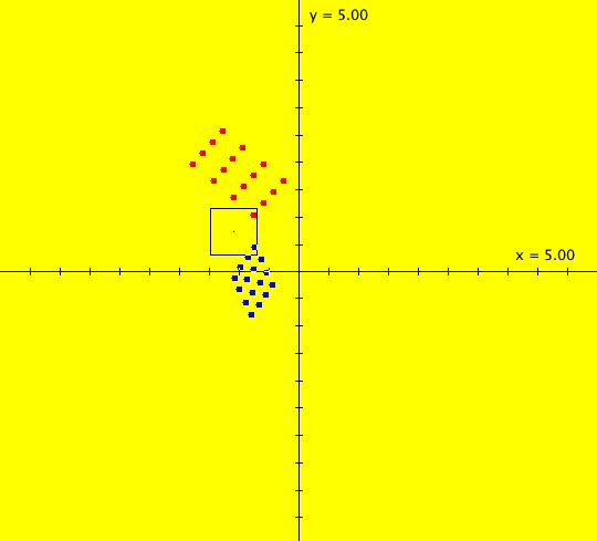
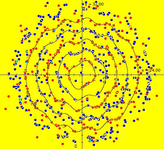
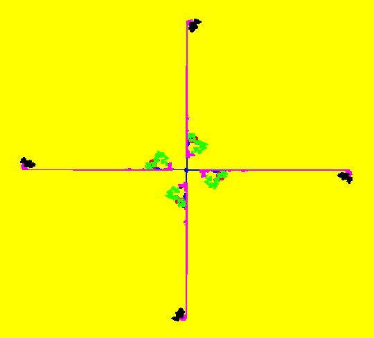
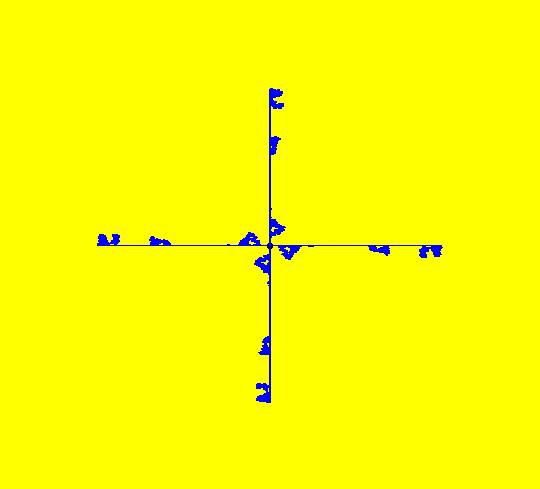
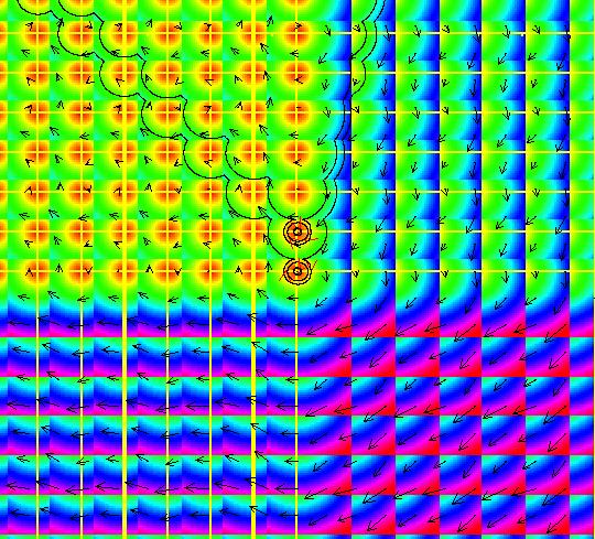
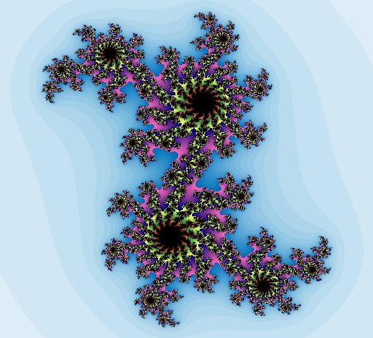
View/Sys/Gal: EMap "( 9j) 2D 169 KAM islands surrounded by chaos IMap0111" in "DynamicalSysExs." This iteration is defined by: x <- y%c-cos(x%b), y <- a-x%c. Parameters are: a = -.430; b = -.210; c = 1.45; This is a variation of ( 9g) where %c is used in both the x and y iterations to constrain the image to a c X c square. There are 13^2 KAM islands surrounded by chaos. Each KAM island is in a 4-island chain. The islands contain periodic orbits with period 4*n where n is a positive integer. Image 1: 169 KAM islands. The last orbit starts at (-0.293268,0.703263) and has period 4. To see the orbit, go to the EMap view and select "Show 2D IMap Orbit Sequence." Image 2: The period of the black orbit (number 175), at x = -0.293, y = 0.703, is 4.
|
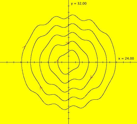
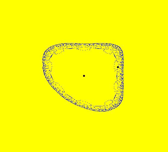
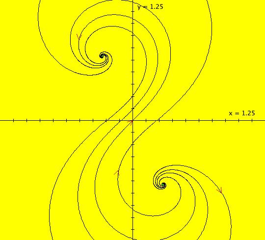
| View/Sys/Gal: Ode "( 9k) 2D the Ode view, an infinity of periodic orbits" in "DynamicalSysExs." This system of odes is defined by the equations: dx/dt = y%c-cos(x%b), dy/dt = a-x%c. Parameters are: a = -.430; b = -.210; c = 1.45; In the view, there are two stable ω-limit cycles. There is also one unstable α-limit cycle (not shown) between them. There is an spiral-out fixed point at the center of the limit cycles.
The unstable α-limit cycle between the inner and outer limit cycles is at about: (x,y) = (-0.204275,0.982153), and has period 2 π. Start a trajectory at the point to see the α-limit cycle. Image 1: A fixed point and two ω limit cycles. Turn the colored vector field on and zoom out 4X. There are an infinite number of fixed points where the nullclines cross at (a-n*c,1+m*c), n and m = 0, 1, . . . and the limit cycle pattern repeats around each of the fixed points. Image 2: Nullcline crossings.
|
|
View/Sys/Gal: Copy of current gallery saved to: "DynamicalSysExs." This iteration is defined by: x <- y-cos(x%b), y <- a-x. Parameters are: a = -.430; b = -.210; There is a single orbit starting at the center of the image: p(0.000000) = (-1.058051,-0.229245). The chaotic orbit stays near p(0) for a while but it leaks out to form an interesting image. Image 1: 10,000 steps. Image 2: 60,000 steps. Open an orbit editor at p(0) and extend the orbit to t = 910,000 to see how it grows. Image 3: 910,000 steps. Start a Flow w/(0,max,120).
|
|
View/Sys/Gal: IMap "( 9m) 2D another example of chaotic leakage, IMap0010" in "DynamicalSysExs." This iteration is defined by: x <- y-cos(x%b), y <- a-x. Parameters are: a = -6.500; b = -6.500; There is a chaotic orbit in the blue region starting at p1 = (-80.708584,-1475.534432) and a period-4 red orbit starting at p2 = (-81.613476,-1475.836949) in the center of the blue region. The blue region is part of a 4-island KAM chain. In this small 5 by 5 view it looks like the blue orbit stays in the island. Image 1: A 5 by 5 view with 10,000 iteration steps. Open the blue orbit's editor then zoom out on the island 3 times and extend the orbit in +t 7 times. Image 2: Blue orbit after +t 6 times. Image 3: Blue orbit after one more +t. We see that the blue orbit leaks out of the island. Is the periodic orbit stable? To find out, extend the periodic orbit in +t 7 times. There is no leakage. We get: p(360000.000000) = (-81.613477,-1475.836950) p(0.000000) = (-81.613476,-1475.836949) For large x and y we can drop the cosine term and parameter "a" so, x <- y-cos(x%b) ~ y and y <- a-x ~ -x. If x and y are large and (x,y) is on the orbit then (-x,-y) is approximately on the orbit. So in the large, the orbits are all approximately parallelograms. Image 4: Parallelograms for large x and y.
|
|
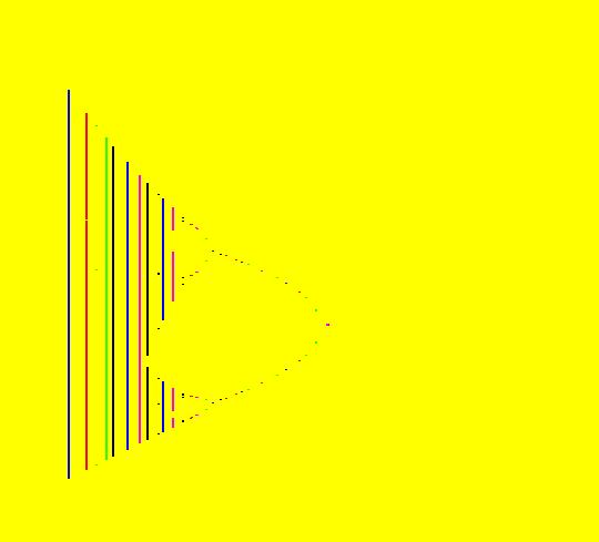
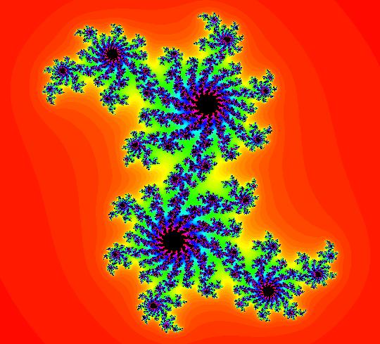
View/Sys/Gal: Ode "(10a) 2D the classic Mandelbrot fractal, EMap as Julia set" in "DynamicalSysExs." This system of odes is defined by the equations: dx/dt = x^2-y^2+p = f(x,y), dy/dt = 2*x*y+q = g(x,y). Parameters are: p = .350; q = .380; Image 1: The EMap view shows a Julia set. Since f(-x,-y) = f(x,y) and g(-x,-y) = g(x,y), if (x,y) is a fixed point then so is (-x,-y) The fixed points of the system are at: 0 = x^2-y^2+.35, 0 = 2*x*y+.38 WA gives the fixed points, (x,y) = +-(-0.288638,0.658264) The Jacobian of the system, in WA notation, is J(x,y) = {{2*x,-2*y},{2*y,2*x}} Entering {{2*x,-2*y},{2*y,2*x}} at x=-.288638, y=.658264 into WA gives eigenvalues: λ = +-(-0.577276+1.316731*i). In the Ode view, six orbits have been started at: (x,y) = (-0.288638,0.658264), (x,y) = (0.288638,-0.658264), (x,y) = (-0.507380,0.828283), (x,y) = (-0.133764,-0.515152), (x,y) = (0.839483,-0.752525) and (x,y) = (0,0). Image 2: The Ode view. As will be shown in system (10d) the AGF generated by the two complex lines: I[1]: (x+0.288638)+i*(y-0.658364) = 0, λ1 = (-0.577276-1.316731*i) and I[2]: (x-0.288638)+i*(y+0.658364) = 0, λ2 = (0.577276+1.316731*i) gives this same system.
|
|
View/Sys/Gal: EMap "(10b) 4D (x^2-y^2+z,2*x*y+w,z,w) EMapCT3 as JSet" in "DynamicalSysExs." This system of odes is defined by the equations: dx/dt = x^2-y^2+z, dy/dt = 2*x*y+w, dz/dt = z, dw/dt = w. The image is the same as the image in system (10a). It looks different because CT3 was used instead of CT0. Shift-click in the graphics area and select CT0 to see for yourself. This system was entered by hand. It is a 4D EMap (x,y) view of a JSet for the 2D system: z <- z^2+c, where c = z0+i*w0. In the (x,y) plane start an orbit was started at: (x,y,z,w) = (0,0,0.35,0.38). You need at least one trajectory in the (x,y) plane to make this work since the EMap algorithm needs a value for (z0,w0), i.e. the value of c. Note that (z0,w0) = (p,q) = (.35,.38) from system (10a).
|
|
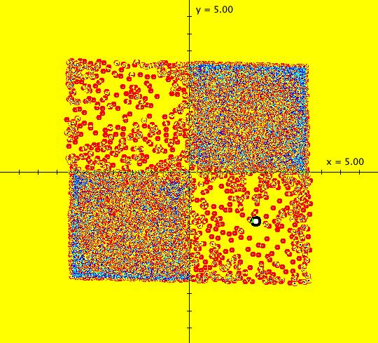
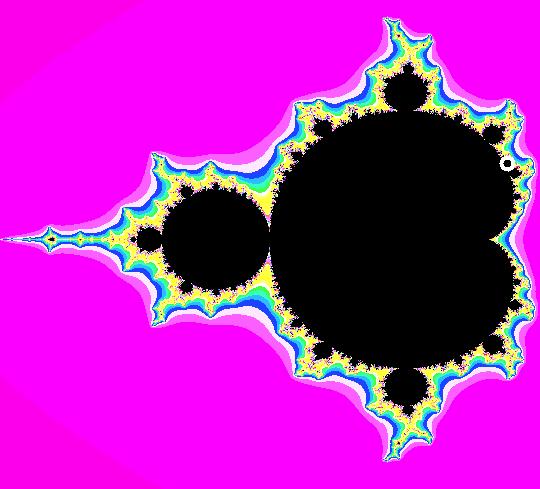
View/Sys/Gal: EMap "(10c) 4D (x,y,z^2-w^2+x,2*z*w+y) 4D EMapCT4 as 2D MSet" in "DynamicalSysExs." This system of odes is defined by the equations: dx/dt = x, dy/dt = y, dz/dt = z^2-w^2+x, dw/dt = 2*z*w+y. The Mandelbrot set for 2D system (10a) dx/dt = x^2-y^2+p, dy/dt = 2*x*y+q can be generated in OdeFactory as follows: (a) starting in system (10a), enter "4D" in the "user fns:" field, update and save the new 4D system (b) in the Ode, or IMap, (x,y) view of the 4D system, set all ICs to 0 then include "EMap" in the 4D system's name Adding "EMap" forces new 4D system to open in the EMap view. This new system is called a "4D companion" of the 2D system (10a). An orbit was started at: (x,y,z,w) = (.35,.38,0,0), on the border of the Mandelbrot set on the right hand edge. To see it, start a Flow. Points on the boundary of the Mandelbrot set correspond to the (p,q) parameter values that give interesting Julia sets. See system (10a) again. Image 1: The black set is the Mandelbrot set. The point (.35,.38) is just off of the upper right edge. System (10b) is another 4D companion system for system (10a). System (10b) shows the Julia set for: (p,q) = (.35,.38).
|
|
View/Sys/Gal: IMap "(10d) 2D the AGF version of (10a), EMap" in "DynamicalSysExs." This AGF is generated by the lines: I[1]: (x+0.288638)+i*(y-0.658264)=0, λ1 = (-0.577276-1.316731*i) I[2]: (x-0.288638)+i*(y+0.658264)=0, λ2 = (0.577276+1.316731*i) Image 1: The EMap view of the system shows a Julia set. The AGF system, which has 16 parameters, is a generalization of the Mandelbrot system which has just 2 parameters. In the Ode/IMap views there are six trajectories/orbits w/ICs: (x1,y1) = (-0.288638,0.658264), (x2,y2) = (0.288638,-0.658264), (x3,y3) = (-0.507380,0.828283), (x4,y4) = (-0.133764,-0.515152), (x5,y5) = (0.839483,-0.752525) and (x6,y6) = (0,0). In the Ode view, ICs (x1,y1) and (x2,y2) correspond to the locations of I[1] and I[2] and they are fixed points. The curved lines are the other 4 Ode trajectories. In the Ode view, the two green dots are handles to the complex generators, I[1] and I[2]. If you click on a green dot, a text-based parameter controller opens and you can change the complex line's 8 parameters. If you shift-click on a green dot a slider-based parameter controller will open. Image 2: The 6 trajectories in the Ode view. In the IMap view, turn on "Show 2D IMap Orbit Sequence" to see the 6 orbits. Image 3: The 6 orbits in the IMap view. Project: Discuss the properties of the trajectories/orbits associated with the 6 ICs in: the Ode, the IMap and the EMap.
|
|
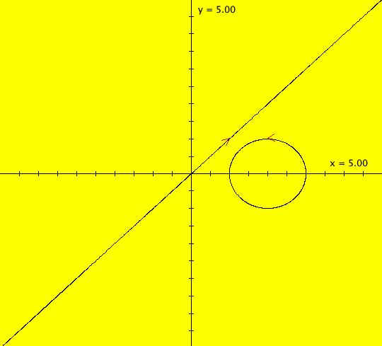
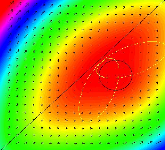
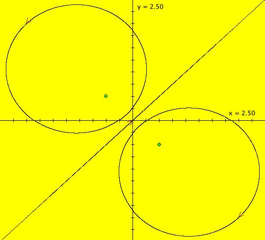
View/Sys/Gal: EMap "(11) 2D quasiHamiltonian system, a line and a circle" in "DynamicalSysExs." This system of odes is defined by the equations: dx/dt = (a*G+b*(2*y)*F), dy/dt = -(a*(-1)*G+b*(2*x-4)*F). Parameters are: a = 1; b = 1; Functions are: F=y-x; G=(x-2)^2+y^2-1 F=0 is the line y = x and G=0 is the circle (x-2)^2+y^2 = 1. These two curves are trajectories for the system of odes for all values of the parameters a and b. Image 1: Two trajectories: (1,1) is on F=0 and (2,1) is on G=0. Image 2: The colored vector field showing the nullcline crossings which are fixed points of the system. Image 3: The EMap view for CT 5. A fractal. In the Ode view, if you vary parameters "a" and b, F=0 and G=0 remain trajectories but the fixed points change. Investigate what happens in the IMap and EMap views.
|
|
View/Sys/Gal: EMap "(12) 2D Robustification of Chaos, EMap" in "DynamicalSysExs." This iteration is defined by: x <- 1-a*(1-c)*x^2+y-a*c*abs(x), y <- b*x. Parameters are: c = .5; a = 1.4; b = .3; EMap CT: 0 Turn "Show 2D IMap Orbit Sequence" on and do a Flow at max speed for 10 seconds. Image 1: Fig. 3 in the 2011 paper by Zeraoulia and Sprott: "Robustification of Chaos in 2D Maps." Get into the IMap view, set hMin = 50, hMax = 150 and go to the 3D/(t,y) view. Turn "Show Approximate Period" on then try adjusting the parameters. See if you can make the chaos "robust" by adjusting c.
|
| View/Sys/Gal: IMap "(13) 2D (-y,x-3*y+y^3), IMap1100" in "DynamicalSysExs." This iteration is defined by: x <- -y, y <- x-3*y+y^3. Blue orbit at (0.764104,0.923093) is a 4-cycle, red orbit at (1,1) is a 2-cycle.
Image 1: IMap 2D/(x,y) view. Image 2: IMap 3D/(t,y) view.
|
|
View/Sys/Gal: Ode "(14a) 2D a symmetric 2-complex-line AGF" in "DynamicalSysExs." This AGF is generated by the lines: I[1]: (x+0.5)+i*(y-0.5) = 0, λ1 = -0.2*i I[2]: (x-0.5)+i*(y+0.5) = 0, λ2 = 0.2*i The degree of the RHS of a 2-complex-line AGF is in general 3. Conjecture: If I[1] is centered at (a,b) and I[2] is centered at (-a,-b) and λ2 = - λ1 then V(x,y) = V(-x,-y) and the 2-complex-line AGF is quadratic. System (14a) in classic "dx,dt, dy/dt" form is: dx/dt = 0.05+x*(0.1*x+0.2*y)-0.1*y^2 dy/dt = 0.05*(1-2*x^2+4*x*y+2*y^2) which is of degree 2. A reflection symmetry about the y = x line reduces the degree from 3 to 2.
|
|
View/Sys/Gal: Ode "(14b) 2D the dx/dt. dy/dt version of AGF (14a)" in "DynamicalSysExs." This system of odes is defined by the equations: dx/dt = 0.05+x*(0.1*x+0.2*y)-0.1*y^2, dy/dt = 0.05*(1-2*x^2+4*x*y+2*y^2).
|
|
View/Sys/Gal: Ode "(15a) 3D finding a strange attractor" in "DynamicalSysExs." This system of odes is defined by the equations: dx/dt = s*(y-x), dy/dt = x*(p-z)-y, dz/dt = x*y-b*z Parameters are: p=28; s=10; b=2.66666 This is the Lorenz system which has a strange attractor. The purpose of the example is to locate the strange attractor using the Monte Carlo method. The trajectory shown was started in the (y,z) plane at: (x(0),y(0),z(0)) = (0.0,6.222222,19.052419). In the (y,z) view, the +x axis is out of the screen directly into your eye. You are viewing the "butterfly wings" more or less perpendicularly. (1) In the (y,z) view, start 100 random dots at .95 of max speed for 20 sec and watch the strange attractor appear (butterfly wings). Dots that leave the view are recreated at random locations in the view. Image 1: The 100 random dots accumulate in the region of the "strange" attractor in the (x,y,z) phase space. (2) To get to the 3D view, select the x button. Try the various 3D subviews. (3) Adjust the parameters p, s and b.
|
|
View/Sys/Gal: Ode "(15b) 3D time-reversal invariance: V -> -V" in "DynamicalSysExs." This system of odes is defined by the equations: dx/dt = -s*(y-x), dy/dt = -x*(p-z)+y, dz/dt = -x*y+b*z. Parameters are: p=28; s=10; b=2.66666 The ICs are the same as in system (15a) but V has been replaced by -V. Time-reversal invariant means that if a vector field V is replaced by -V then the +t part of the V trajectories will be the same as the -t parts of the -V trajectories and vice versa. For (15a): p(9.331200) = (6.528890,11.588659,13.027594) p(0.000000) = (0.000000,6.222222,19.052419) p(-0.227710) = (-43.645613,-13.492224,18.443635) For (15b), the time reversed version of (15a): p(0.227710) = (-43.645613,-13.492225,18.443636) p(0.000000) = (0.000000,6.222222,19.052419) p(-9.331200) = (6.526878,11.585747,13.024092) A trajectory starts at the same point in (15a) and (15b) but time is reversed so the arrowheads point in opposite directions and final +t and -t points are reversed. Image 1: The Monte Carlo method applied in the -t direction to (15b).
|
|
View/Sys/Gal: Ode "(15c) 3D you can't go home again if the system is chaotic" in "DynamicalSysExs." This system of odes is defined by the equations: dx/dt = s*(y-x), dy/dt = x*(p-z)-y, dz/dt = x*y-b*z. Parameters are: p=28; s=10; b=2.66666 This trajectory was started at the +t end of the trajectory in system (15a): last (x,y,z,t) = (6.528889571846378, 11.588659053740995, 13.027594491465589, 9.3311999999921). For this system, the graphics area is the x = 6.528889571846378 plane and the starting point for the trajectory is (x(0),y(0),z(0) = (6.528889571846378, 11.588659053740995, 13.027594491465589). When the trajectory is extended in -t, it does not return to the start of system (15a) trajectory because: (a) you cannot really find the "exact" +t end of the system (15a) trajectory and (b) the system is chaotic so if you don't start at the exact +t end you will not return to the starting point going backwards in time. Mathematically, the system is time-reversal invariant (replacing t by -t in the system gives the same trajectory when you start at the same point in R3) but in practice, because the system is chaotic, it is not time-reversal invariant if you start at the +t end of a trajectory in R3 and reverse time to get back to the starting point. Image 1: The arrowhead is at the t0 point on the (15c) trajectory and on the +t end of the (15a) trajectory but the -t part of the (15c) trajectory does not return to the starting point of the (15a) trajectory.
|
|
View/Sys/Gal: Ode "(16) 4D simulating projectile motion" in "DynamicalSysExs." "Flow" animations were implemented in OdeFactory to provide a tool that can be used to visualize the global dynamic properties of dynamical systems. When the systems serve as models of physical systems, the animations are animations of the physical systems. Shoot a projectile at various values of the angle of elevation and watch it fly. The classic way to find the equations of motion for the 2D projectile motion problem (no cross wind), without drag (no air resistance), is to start with the Hamiltonian function. Set the mass m = 1 then, assuming energy is conserved (no drag), the Hamiltonian for the system is H = v^2/2+g*y. Let v in x dir = vx = dx/dt = z, v in y dir = vy = dy/dt = w so H = (z^2+w^2)/2+g*y and the equations of motion are dx/dt = Hz = z, dy/dt = Hw = w, dz/dt = -Hx = 0, dw/dt = -Hy = -g Parameters are: g=32 Set z(0) = w(0) = 200/sqrt(2) = 141.4 ft/sec for max range. x is the horizontal position in feet y is the vertical position in feet z is the horizontal velocity in ft/sec, z(0) = 141.4 w is the vertical velocity in ft/sec, w(0) = 141.4 The (x,y) view shows the trajectory of a projectile shot first at 45 degrees then at 30 degrees, where z(0) = 173.2, w(0) = 100, with an initial velocity of 200 ft/sec. To find out approximately how long the projectile is in the air for each trajectory, set the lower limit on the y axis to -1, i.e. "vMin" = -1, close the border (click the red "Bdr" button) then click in the graphics area on the arrowheads at (x,y) = (0,0). You will see that for the first trajectory the projectile is in the air about 8.84 sec and that the second trajectory it is in the air for about 6.26 sec. (1) Do a "Flow" animation at .95 of max speed for 30 seconds and watch the flight of the projectiles.
|
An OdeFactory Slide Show Click on a slide to zoom in. Click "video" to see a video.
|
View/Sys/Gal: Ode "Appendix 1: Time - Dynamical Systems - Computer Simulations" in "DynamicalSysExs." ======================================= ===== Time passes, things change. ===== ======================================= The concept of time, and its relationship to change and motion, can be viewed from the point of view of: Philosophy or Physics or Mathematics or Computer Science. For a historical philosophical overview of the concept of time see: "The Philosophy of Time". For a contemporary discussion of time by a Cosmologist, a Philosopher of Physics, a Computer Scientist and a Neuroscientist, see "Understanding How Time Works, from Cosmology to Cognition." (55 min video) There is another good discussion of time called A Matter of Time. Time intrinsically involves change. Physical motion is the change of something in some medium. Aristotle thought of time as the measure of motion. To Aristotle space was real and continuous, and time was continuous but not real. From the Physics, Mathematics and Computer Science points of view, OdeFactory simulates the time-evolution of points in the state space of an abstract dynamical system. ======================================= ======= ~ Historical Timeline ======== ======================================= 350BC Aristotle: reality, time, motion continuity 1670s Newton: trying to understand nature calculus, "solving" odes, F = m*a 1890s (Newton+220yrs) Poincare: most odes can't be "solved" trying to understand odes globally geometry, phase space 1940s (Poincare+50yrs) Computers: numerical "solutions" of odes
1960s (Computers+20yrs) Lorenz: studied a small weather model got strange computation results strange attractors, chaos 1970s (Lorenz+10yrs) Feigenbaum: trying to understanding chaos iteration maps phase transitions and chaos "Feigenvalues" 1980s (Feigenbaum+10yrs) Mandelbrot: used the escape-time algorithm trying to understand fractals defined non-integer dimensions ======================================= === Physics, Math, Computer Science === ======================================= Physical Dynamical Systems: Physics: experiment + math -> laws Abstract Dynamical Systems: Math: axioms + logic -> theorems Computer Simulation of Dynamical Systems: machine + algorithms -> motion ======================================= ====== Abstract Dynamical System ====== ======================================= There are various mathematical definitions of an Abstract Dynamical System: "A dynamical system is a concept in mathematics where a fixed rule describes the time dependence of a point in a geometrical space." (1st definition). Or "A dynamical system is a rule for the time evolution of a state space." (2nd definition). Abstract Dynamical System = State Space + "Time" + Evolution Algorithm. The Evolution Algorithm maps points in the state space to points in the state space. The state space is Rn. For odes the "evolution" may be forward or backward in time. For odes "time" is continuous for maps it is discrete. ======================================= ===== Ex: Real Dynamical System ======= ======================================= In order to gain a better understanding of the relationships between real dynamical systems, abstract dynamical systems and computer simulations of dynamical systems, consider the example of a mass on a spring. (the Physics Classroom) The state space of the abstract system, R2, consists of the position and velocity of the mass. If the real mass is displaced some initial distance from the equilibrium position, and released, it moves back and forth about the equilibrium position. If we are the mass, we can experience the motion directly, but we cannot know our exact location in the abstract phase space. This is because quantum mechanics tells us that we cannot simultaneously know both the position and velocity of an object with complete certainty. So - the real state space is a fuzzy version of the abstract state space, R2. Quantum mechanics also tells us that we cannot simultaneously know the time and energy of a system so real "time" is not simply a point on the real line R. Furthermore, special relativity changes the meaning of time altogether so the relationship between a real dynamical system and an abstract dynamical system becomes a bit nebulous. ======================================= ==== Ex: Abstract Dynamical System ==== ======================================= Abstract dynamical systems, defined as "a concept in mathematics" or "a rule for the time evolution on a state space," are symbolic (language based) representations of change or motion. The mass-on-a-spring abstract dynamical system, with mass m and spring constant k, consists of: the State Space = R2, with position x and velocity y: p(0) = (x(0),y(0)) and "Time" = t ∈ R1 an Evolution Algorithm, Newton's 2nd Law, F=ma: F = -k*x = m*a = m*x'' or -k*x/m = x'', let y = x' then y' = x'' = -k*x/m
so we get dx/dt = y, dy/dt = -k*x/m. We can include a "display" algorithm (a) symbolic alg: WA applied to: dx/dt = y, dy/dt = -k*x/m, x(0) = 1, y(0) = 0 gives the continuous functions x(t) = cos(C*t), y(t) = -C*sin(C*t)) where C = sqrt(k/m) (b) or numerical alg: RK4 gives the approximate points p(0), ~p( Δt), ... ~p(n* Δt) where Δt = .01 The abstract definition of a dynamical system is a mathematical description of motion. It enables us to prove theorems about motion but it does not enable us to see the motion directly. To see motion or change we need a real physical system or a computer simulation of the abstract system. ======================================= ========= Computer Simulation ========= ======================================= Digital Computer = Store (program & data) + CPU (Arithmetic/Logic Unit) + Clock + Fetch/Execute Cycle Computer Program = Input = Initial State of Store + Clock Cycle, Execution Cycle + Algorithm(s) -> Output = New State of Store A computer can only compute a finite sequence of steps defined by an algorithm that modifies the data store. Consequently it can only simulate the motion defined by an abstract dynamical system. The computer also uses a finite discrete subset of the real numbers and a discrete display system so the sequence of points computed and displayed can only be approximately correct. A real dynamical system is not the same as an abstract dynamical system which in turn is not the same as a computer simulation of an abstract dynamical system.
|
An OdeFactory Slide Show Click on a slide to zoom in. Click "video" to see a video.
|
View/Sys/Gal: Ode "Appendix 2: OdeFactory: Time, Terms and Observations" in "DynamicalSysExs." ======================================= ======== Time in OdeFactory =========== ======================================= In OdeFactory the fixed rule, called a vector field, consists of a list of algebraic expressions (algorithms). The length of the list, n, where n <= 4, is the dimension of the phase space which mathematically is Rn. In OdeFactory Rn is approximated by n-tuples of 64-bit IEEE floating point numbers. The vector field dynamically distorts the phase space by mapping points in Rn into points in Rn. The vector field, applied stepwise to successive values of an initial point, generates a sequence of points in the phase space. In the Ode view, each step, called a "time" step, advances the point a very small distance (a few pixels on the computer screen) in the phase space so the point appears to move on a continuous curve called a trajectory. For a 2D system, the phase space is R2, that is the (x,y) plane, and the extended phase space is R3, the 3D space (t,x,y). In the Ode view, the sequence of points generated by the dynamical system in the extended phase space is called a solution curve. A trajectory in the phase space is the projection of solution curves in (t,x,y) onto (x,y). The dynamics, or motion, associated with a dynamical system occurs in the phase space, not in the extended phase space. In the discrete time IMap view, each iteration step advances the point a large distance (one time step and many pixels on the computer screen). In the phase space the motion is no longer continuous but instead appears to hop along in a sequence of discrete jumps between points in the phase space. For an IMap, the sequence of discrete points is called an orbit. To better follow the time sequence of points OdeFactory includes options to connect the points and/or to animate the sequence. In all views, "time" is just a measure of the length of an ordered sequence of events. A real-time animation is one that simulates the motion defined by a dynamical system - as the motion is computed. Real-time animations can be created in OdeFactory by using the "Flow" button in the "Graphics Settings" window. The animations are implemented by using threads in Java. ======================================= ======= OdeFactory Terminology ======== ======================================= * fixed rule ("law" of motion) > t-advancing map: Rn ? Rn > n algebraic expressions, ex: "y" and ""-k*x/m, n = 2 > n algorithms, ex: "y" and "-k*x/m," n = 2 > n dimensional vector field, ex: V = (y,-k*x/m) > control parameters, ex: k and m * geometrical space > phase space = Rn, ex: R2 = (x,y) plane > trajectories/orbits in Rn > extended phase space = R ? Rn * time = sequence of steps in an algorithm > continuous, RK4, Δt = +-.01 gives the Ode view > discrete, Δt = +1 only gives the IMap/EMap views * motion > "real-time" simulated motion > time-lapse animation * control parameters > not part of the phase space > new parameter => new system > can be "promoted" to phase space ======================================= ========= Some Observations =========== ======================================= Computer programs themselves are dynamical systems. They have a complex fractal structure (algorithms within algorithms), they are nonautonomous (can have real-time inputs from the user) and they are chaotic (small changes can make big differences). OdeFactory can be thought of as an interactive meta-dynamical system designed to support virtual mathematics. A Chinese proverb: Tell me, I'll forget. Show me, I'll remember. Involve me, I'll understand. Aristotle: For the things we have to learn before we can do them, we learn by doing them.
| ||||||||||||||||||||||||||||||||||||||||||||||||||||||||||||||||||||||||||||||||||||||||||||||||||||||||||||||||||||||||||||||||