Click on an image to go directly to a system or scroll to see all of the systems in this gallery.
 |
 |
 |
 |
 |
 |
 |
 |
 |
 |
 |
 |
 |
 |
 |
 |
 |
 |
 |
 |
 |
 |
 |
 |
 |
 |
 |
 |
 |
 |
 |
 |
 |
 |
 |
 |
 |
 |
 |
 |
 |
 |
 |
 |
 |
 |
 |
 |
 |
 |
 |
 |
 |
 |
 |
 |
 |
 |
 |
 |
 |
 |
 |
 |
 |
 |
 |
 |
 |
 |
 |
 |
 |
 |
 |
 |
 |
 |
 |
 |
 |
 |
 |
 |
 |
 |
 |
 |
 |
 |
 |
 |
 |
 |
 |
 |
 |
 |
 |
 |
 |
 |
 |
 |
 |
 |
 |
 |
 |
 |
 |
 |
 |
 |
 |
 |
 |
| OdeFactory Images and Annotations | |||||||||||||||||||||||||||||||||||||||||||||||||||||||||||||||||||||||||||||||||||||||||||||||||||||||||||||||||||||||||||||||||||||||||||||||||||||||||||||||||||||||||||||||||||
|
|
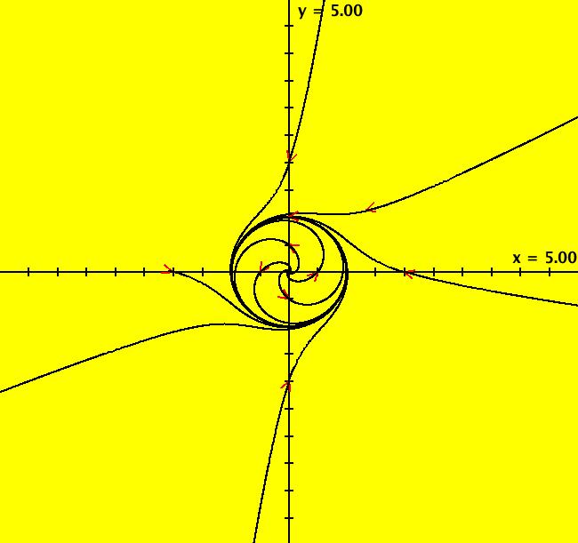
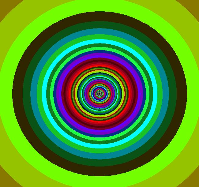
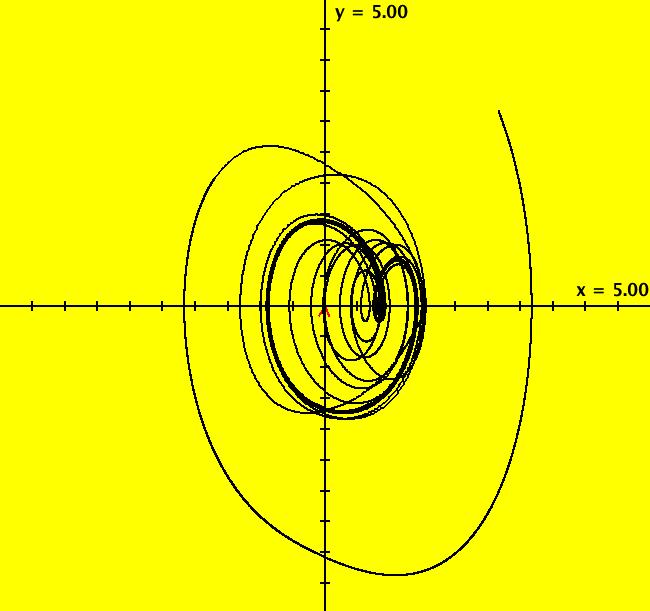
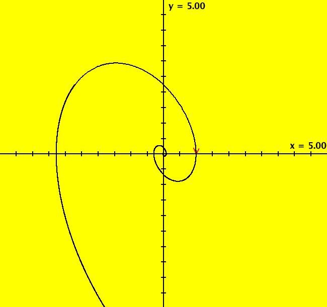
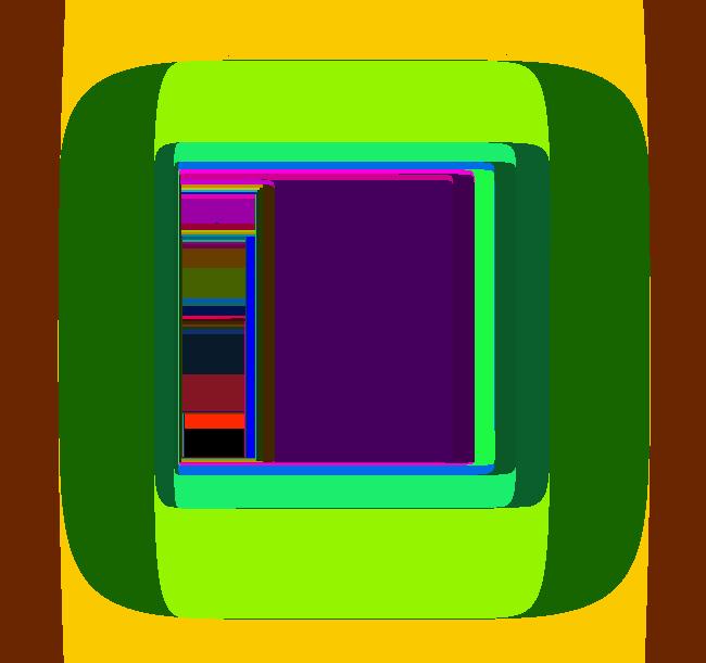
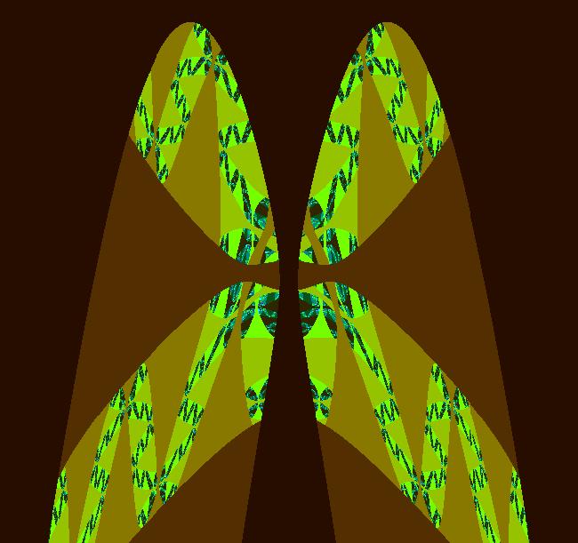
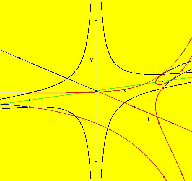
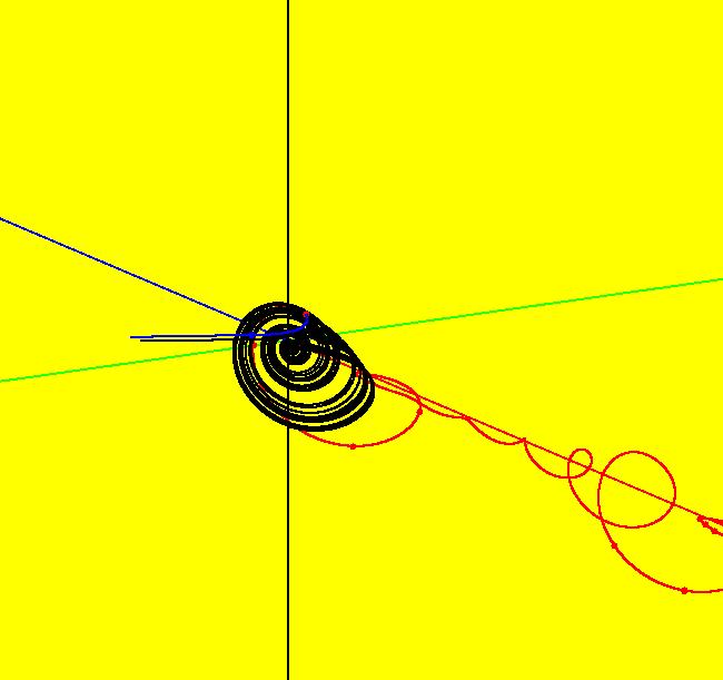
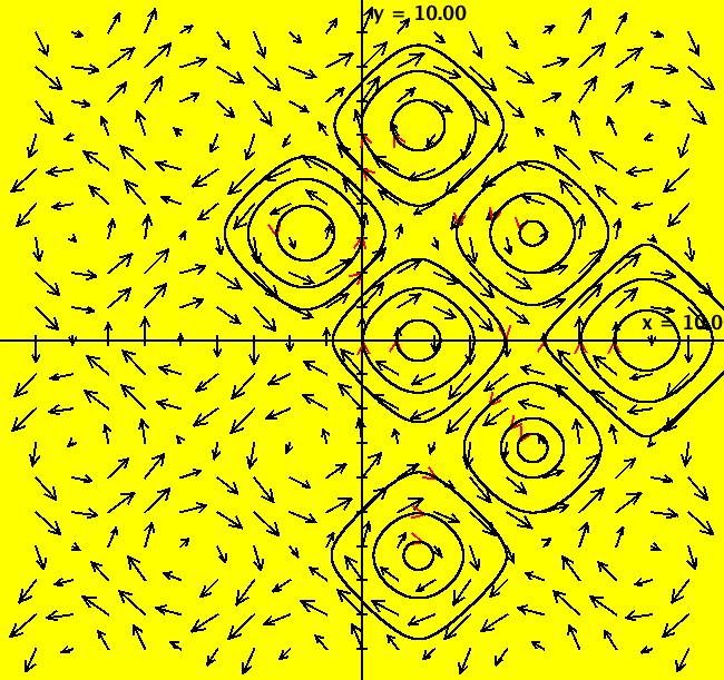
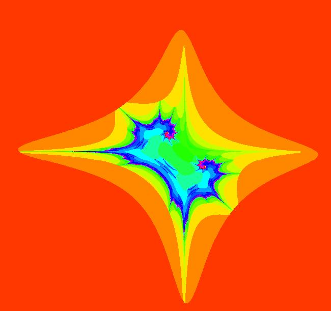
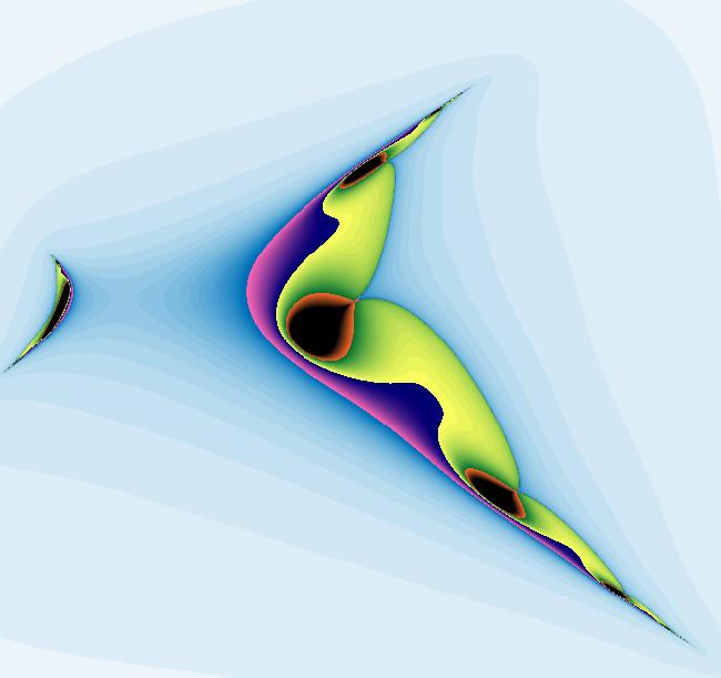
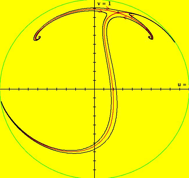
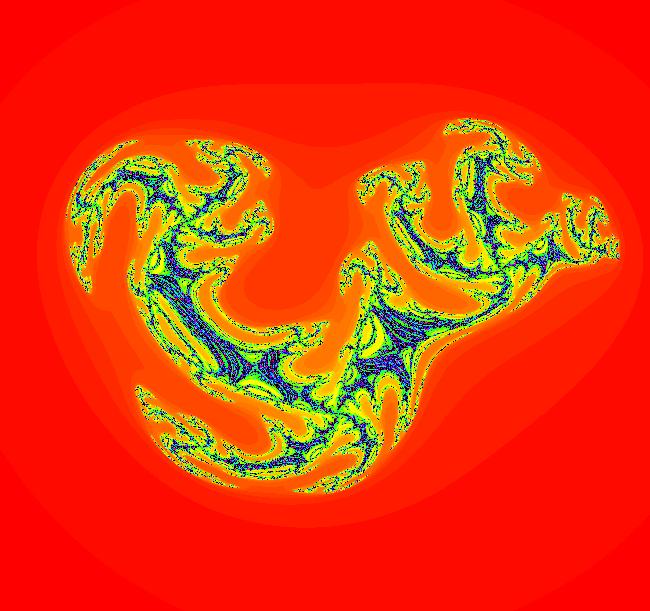
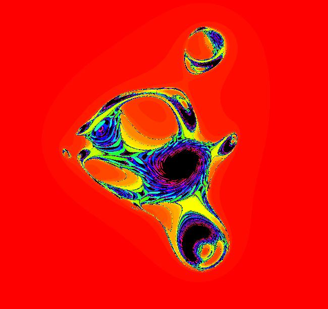
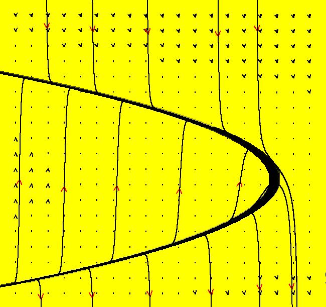
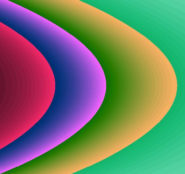
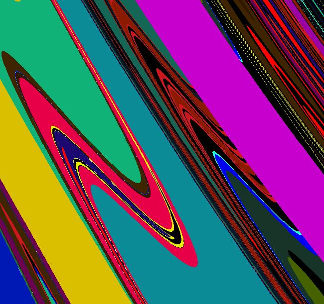
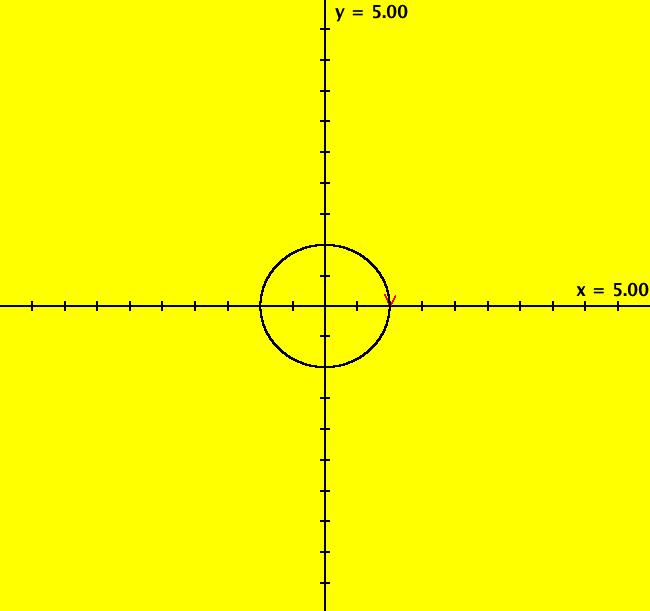
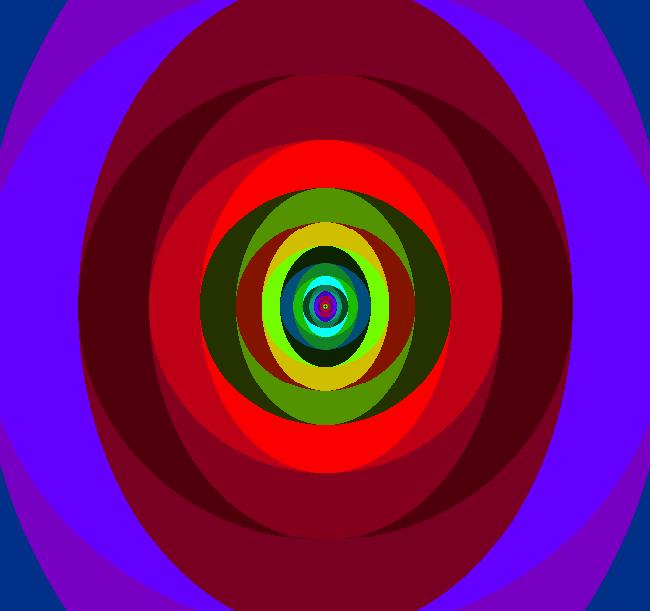
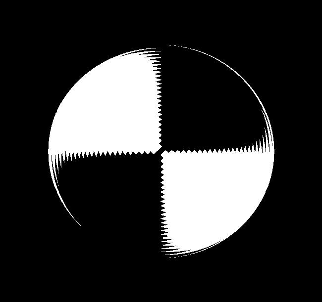
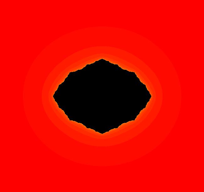
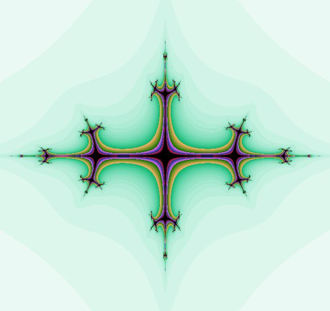
View/Sys/Gal: Ode "Andronov-Hopf bifurcation" in "OdeFactoryExs." This system of odes is defined by the equations: dx/dt = b*x-y-x*R, dy/dt = x+b*y-y*R Parameters are: b = 1 Functions are: R = x^2+y^2 The trajectory starting at (0,1) is a periodic orbit with period 2* π. Select "Show Approximate Orbit Period" on the Help menu to calculate the period. Clear the view and start a single trajectory then click on the "Adj Ctrl Params..." button then drag the slider around to change the control parameter b. For further details concerning this system, see: Andronov-Hopf bifurcation. Image 1: Ode view in R2+. Image 2: Ode view in 3D. Clear, then click, Flow button. Reopen then view as an IMap while changing b. Image 3: EMap view with b = 2.1, zoomed in.
|
||||||||||||||||||||||||||||||||||||||||||||||||||||||||||||||||||||||||||||||||||||||||||||||||||||||||||||||||||||||||||||||||||||||||||||||||||||||||||||||||||||||||||||||||||
|
|
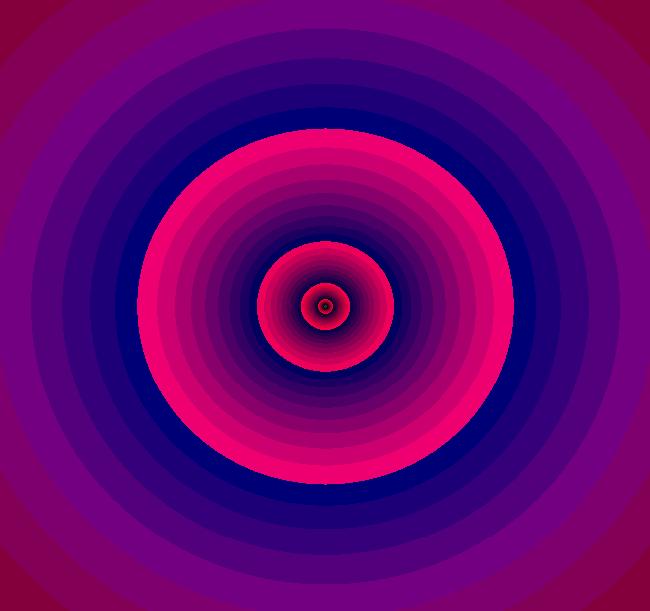
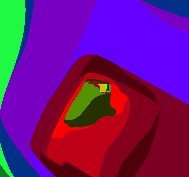
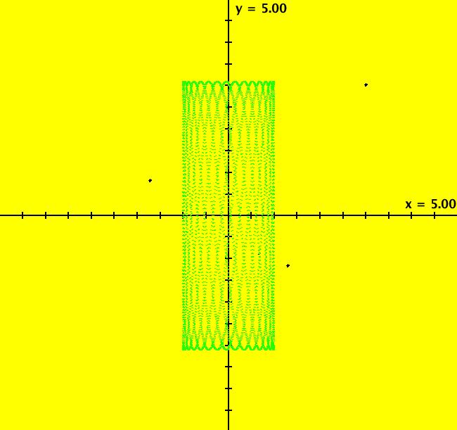
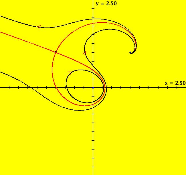
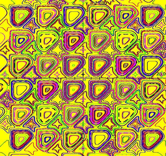
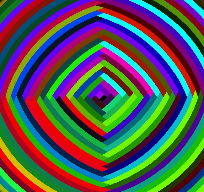
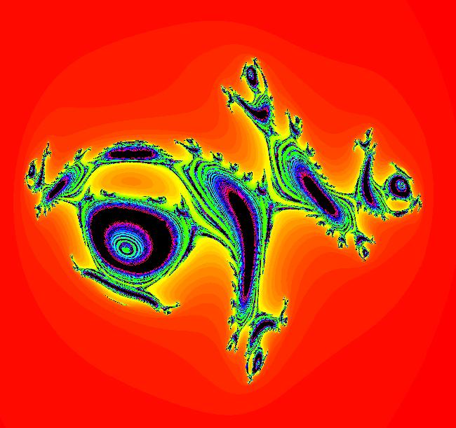
View/Sys/Gal: EMap "Andronov-Hopf bifurcation EMapCT2" in "OdeFactoryExs." This iteration is defined by: x <- b*x-y-x*R, y <- x+b*y-y*R. Parameters are: b = -.300; Functions are: R = x^2+y^2 Image 1: EMap CT: 2 view.
|
||||||||||||||||||||||||||||||||||||||||||||||||||||||||||||||||||||||||||||||||||||||||||||||||||||||||||||||||||||||||||||||||||||||||||||||||||||||||||||||||||||||||||||||||||
|
|
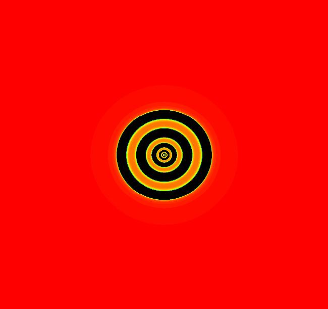
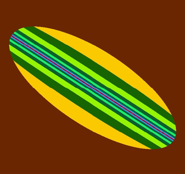
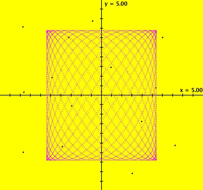
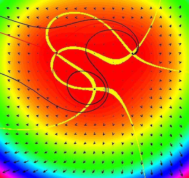
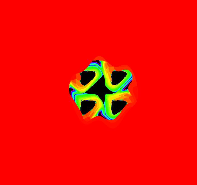
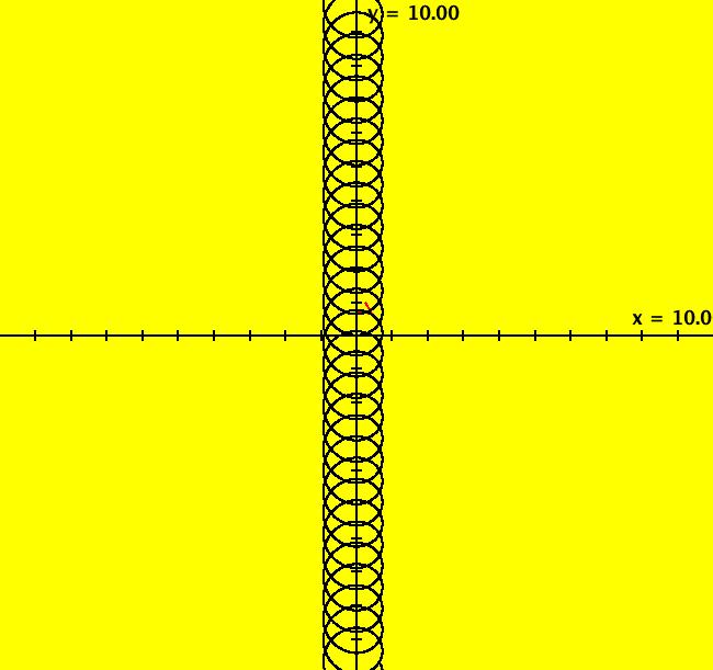
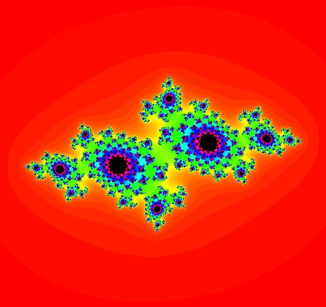
View/Sys/Gal: EMap "Andronov-Hopf bifurcation EMapMaxCT6" in "OdeFactoryExs." This iteration is defined by: x <- b*x-y-x*R, y <- x+b*y-y*R. Parameters are: b = -.5000; Functions are: R = x^2+y^2 Image 1: EMapMax CT: 6 view.
|
||||||||||||||||||||||||||||||||||||||||||||||||||||||||||||||||||||||||||||||||||||||||||||||||||||||||||||||||||||||||||||||||||||||||||||||||||||||||||||||||||||||||||||||||||
|
|
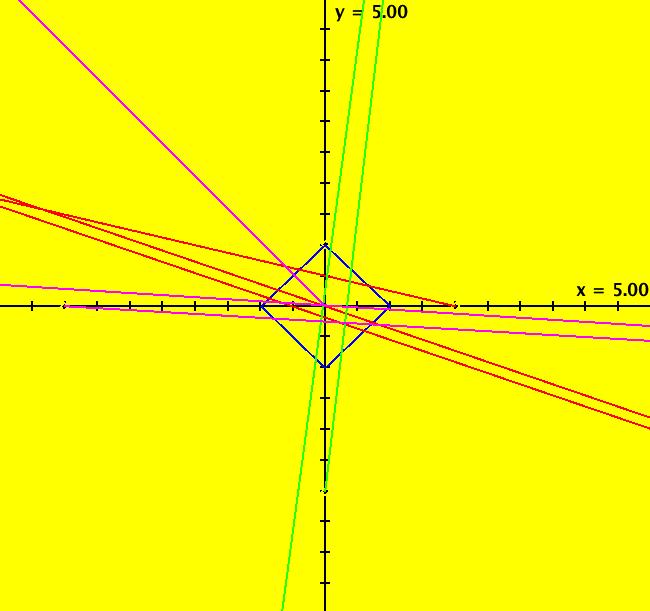
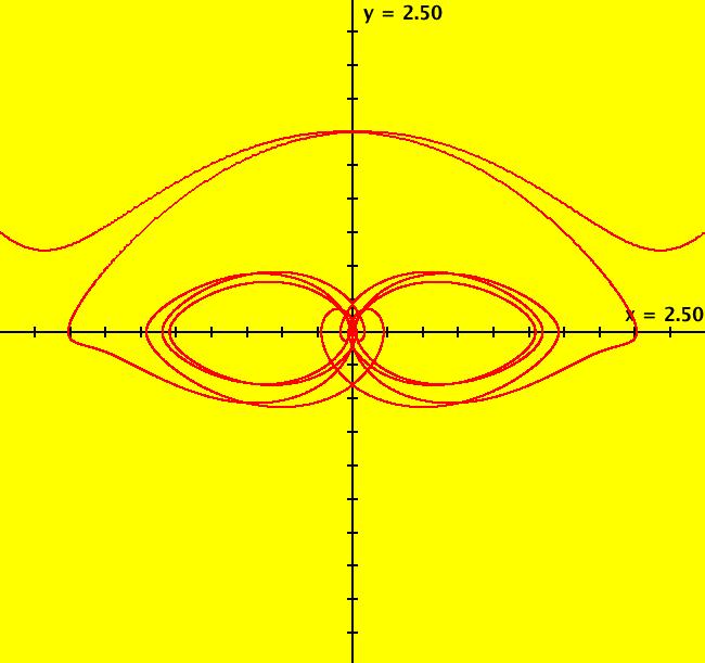
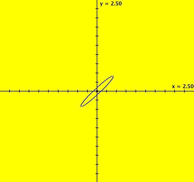
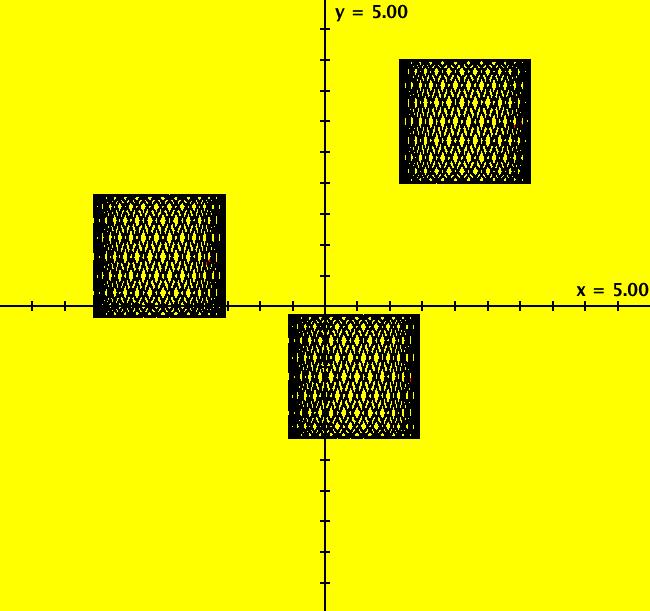
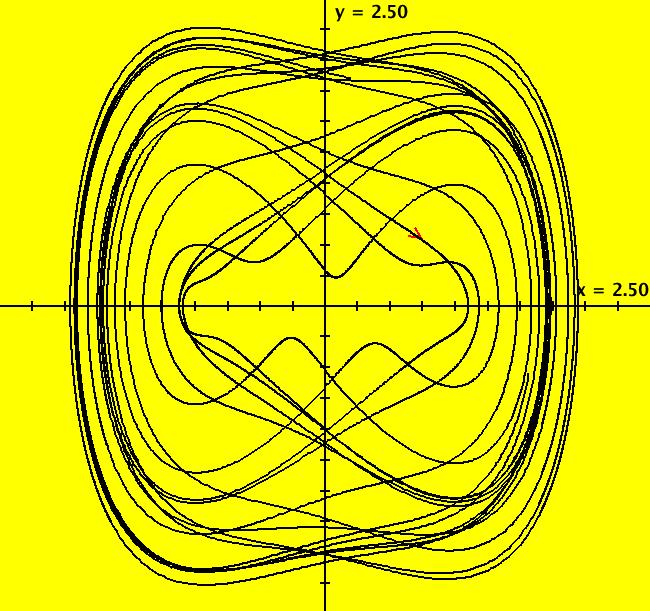
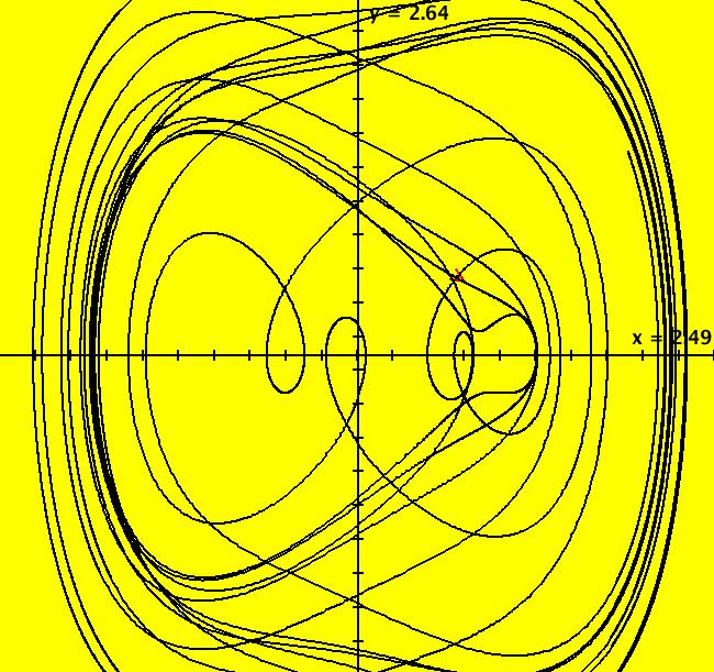
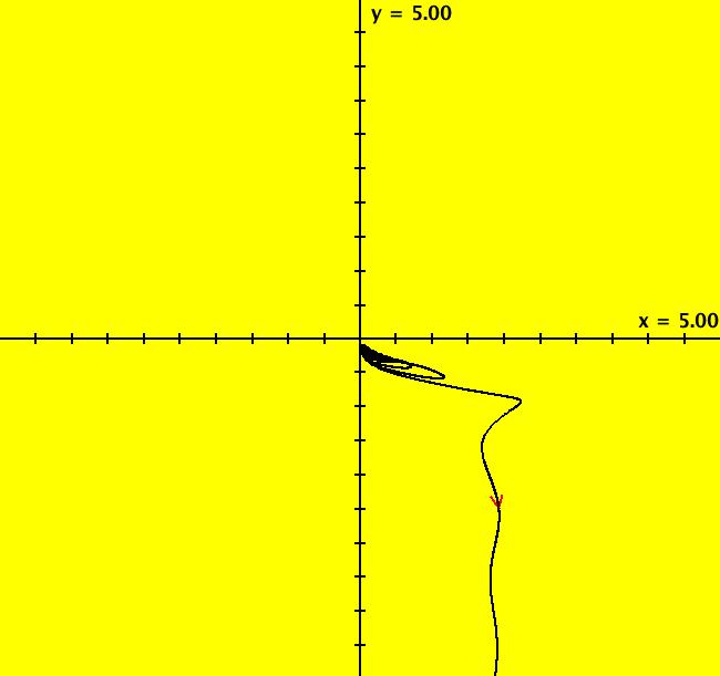
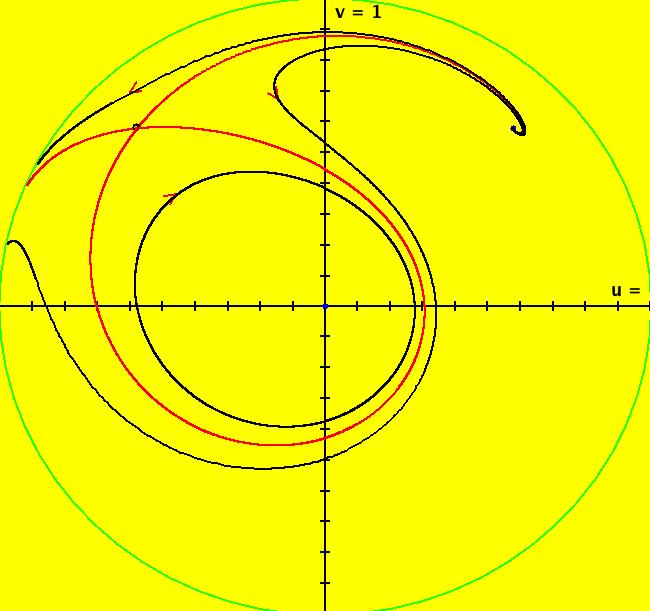
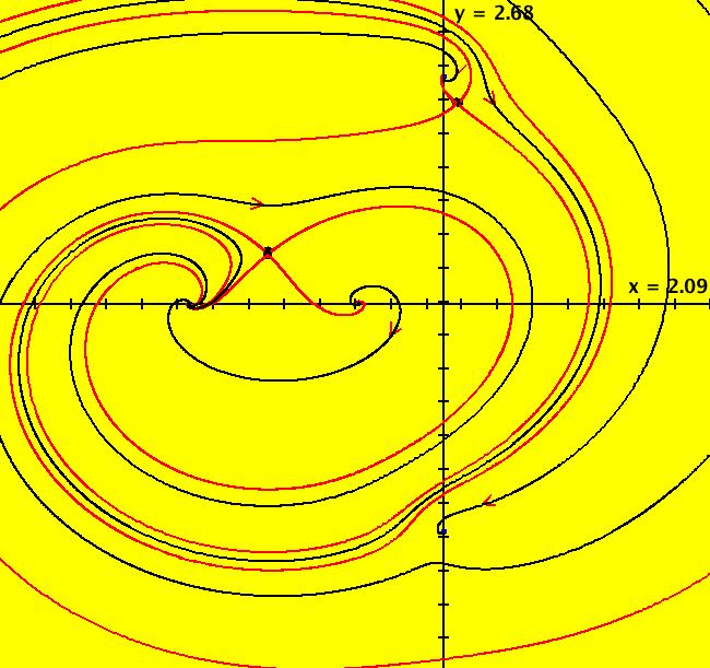
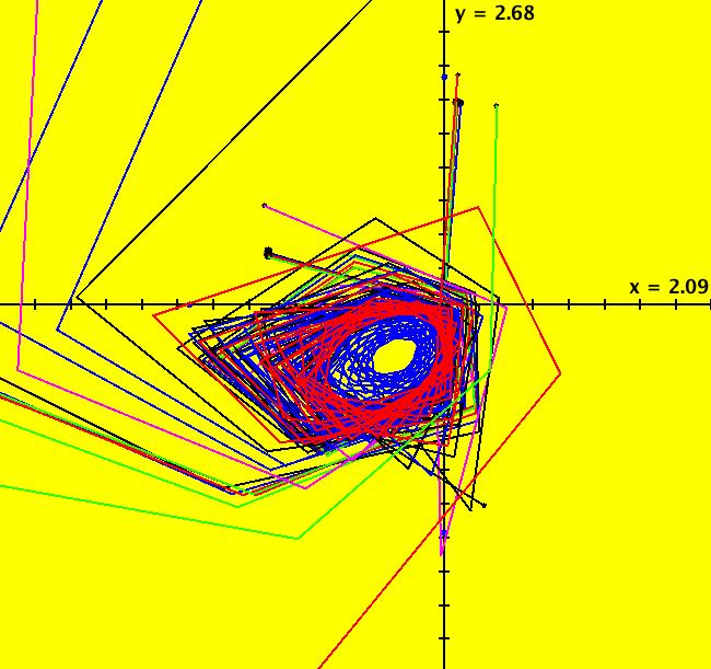
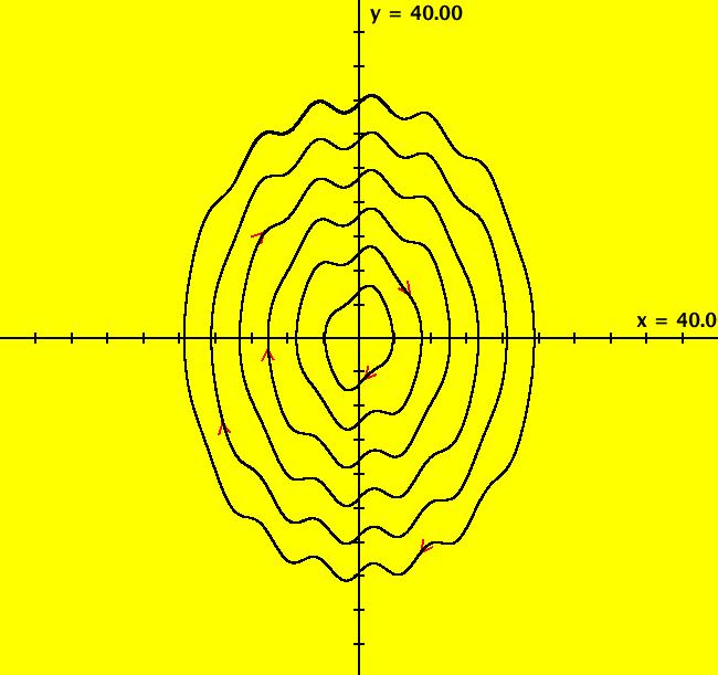
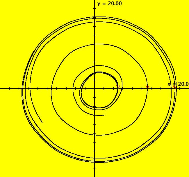
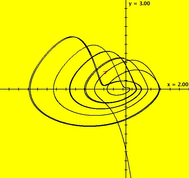
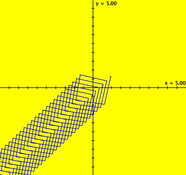
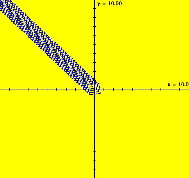
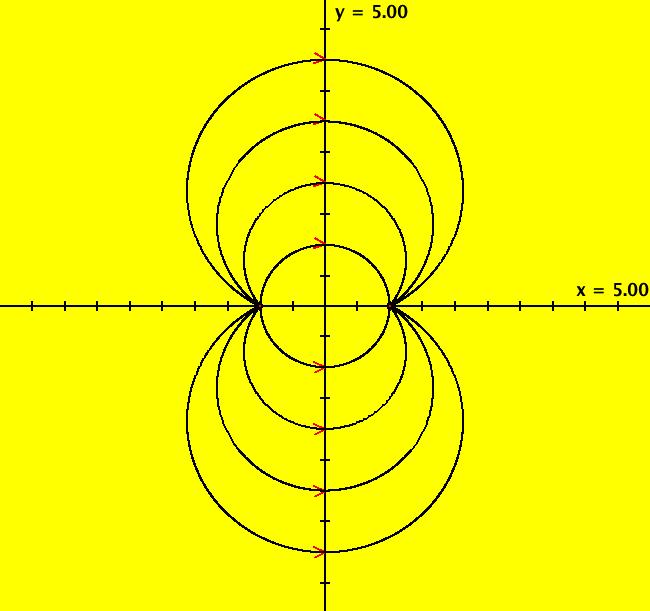
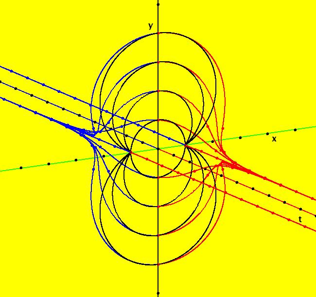
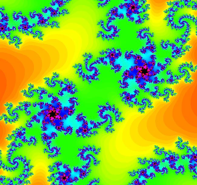
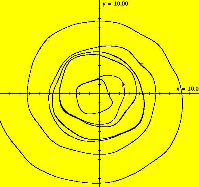
View/Sys/Gal: IMap "Andronov-Hopf bifurcation IMap1000" in "OdeFactoryExs." This iteration is defined by: x <- b*x-y-x*R, y <- x+b*y-y*R. Parameters are: b = 1; Functions are: R = x^2+y^2 Image 1: EMap view for b = 2.1. In the Ode view, for each point p = (x,y) there is a b > 0 such that the trajectory starting at p is a limit cycle which is a circle of radius sqrt(b). In the IMap view the situation is more complicated. Some seeds are on cycles for some values of b > 0. For example:
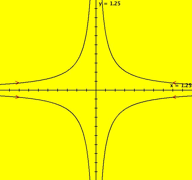
Image 2: IMap view for b = 1.
|
|
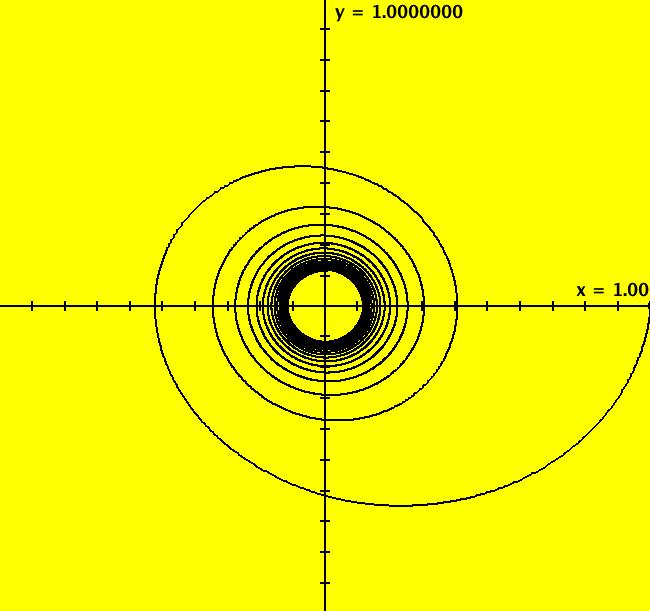
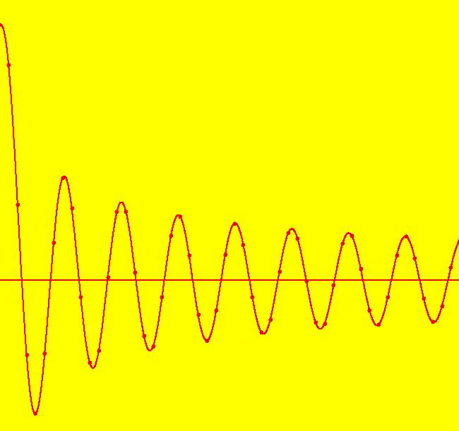
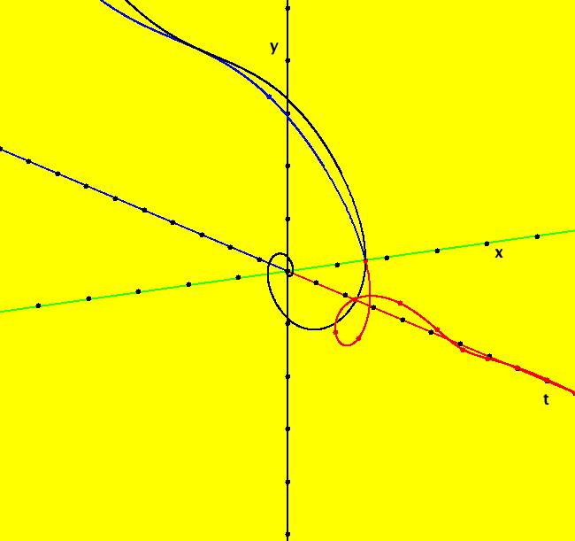
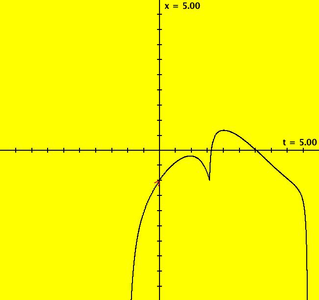
View/Sys/Gal: Ode "Bessel equation" in "OdeFactoryExs." This system of odes is defined by the equations: dx/dt = y, dy/dt = -y/t-(1-1/t^2)*x, t != 0 in the (t,x,y) coordinate system, and the ICs are (x(1),y(1))=(1,0). The 1st order 2D system corresponds to the 2nd order ode y'' = -y'/x-(1-1/x^2)*y, x != 0 or x^2*y''+x*y'+(x^2-1)*y = 0 in the (x,y) coordinate system, and the ICs are (y(1),y'(1)=(1,0). The solution curve in the (x,y) system is y(x), which in the (t,x,y) system, is shown in the 3D/(t,x) view. Drop y'' = -y'/x-(1-1/x^2)*y, y(1) = 1, y'(1) = 0 into WA to check the results. Image 1: The image is the trajectory for the 1st order system with ICs (x(1),y(1))=(1,0) in the (x,y) phase space or the y' vs y curve for the 2nd order ode in normal form. Image 2: Updating (vMax,vMin) to (1.1,-.6) and (hMin,hMax) to (1,52) and going to the 3D/(t,x) view shows x(t) for the system or, y vs x for the 2nd order ode in normal form.
|
|
View/Sys/Gal: Ode "Duffing's equation" in "OdeFactoryExs." This system of odes is defined by the equations: dx/dt = y, dy/dt = -.2*y+x-x^3+.3*cos(t) in the (t,x,y) coordinate system. The 1st order 2D system corresponds to the 2nd order ode y'' = -.2*y'+y-y^3+.3*cos(x) in the (x,y,y') coordinate system. ICs are (t,x,y) = (0,0,0). The trajectory has been extended to t about 4000. Image 1: Get into the 3D/(x,y) view to see the PMap (Poincare map or section). Return to the phase space, clear the view, then start a trajectory at (0,0). Click on the Flow... button and start 20 random dots. After the animation stops, zoom out twice then select the t button (in addition to the x and y buttons) to see the solution curve in the extended phase space. See: Duffing oscillator.
|
|
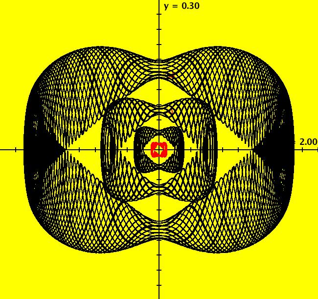
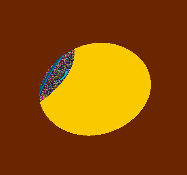
View/Sys/Gal: EMap "Duffing's equation, another form" in "OdeFactoryExs." This system of odes is defined by the equations: dx/dt = y, dy/dt = -x+x^3/6+.8*sin(.27*a*t) in the (t,x,y) coordinate system. The 1st order 2D system corresponds to the 2nd order ode y'' = -y+y^3/6+.8*sin(.27*a*x) in the (x,y,y') coordinate system. Parameters are: a=.92845 Image 1: Ode view. ICs are: x(0)=y(0)=0 Image 2: IMap view. The blue ring is a global attractor. Image 3: EMap view, zoomed out once, of the prisoner set. Click on the CPs... button and try some values of "a" near 1. See: p. 221, ex 11 of "Numerical Solution of Differential Equations" by Isaac Fried. See Fig. 9.18, p. 222, of Fried. Note Fried gets 3 maxs before x(t) --> inf. Try a = 9283 to get better agreement with Fried's result. Conclusion: this ex is not stable in the value of parameter "a."
|
|
View/Sys/Gal: Ode "Duffing's equation, autonomous form" in "OdeFactoryExs." This system of odes is defined by the equations: dx/dt = 1, dy/dt = z, dz/dt = -.2*z-y*abs(y)+1.5*cos(2*x)+.5 Image 1: The Ode 3D/(t,y,z) view with ICs (x,y,z) = (0,0,0).
|
|
View/Sys/Gal: Ode "Duffing's equation, nonautonomous form" in "OdeFactoryExs." This system of odes is defined by the equations: dx/dt = y, dy/dt = -.2*y-x*abs(x)+1.5*cos(2*t)+.5 in the (t,x,y) coordinate system. The 1st order 2D system corresponds to the 2nd order ode y'' = -.2*y'-y*abs(y)+1.5*cos(2*x)+.5 in the (x,y,y') coordinate system. Image 1: Ode view with ICs x(0)=y(0)=0. See: p. 221, ex 10 of "Numerical Solution of Differential Equations" by Isaac Fried.
|
|
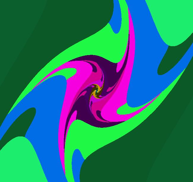
View/Sys/Gal: EMap "Duffing's equation, nonautonomous form, EMapCT2" in "OdeFactoryExs." This iteration is defined by: x <- y, y <- -.2*y-x*abs(x)+1.5*cos(2*t)+.5. EMap CT: 2 Image 1: EMap view. This image is a fractal. Zoom in/out.
|
|
View/Sys/Gal: EMap "Fibonacci sequence as an EMapCT5" in "OdeFactoryExs." This iteration is defined by: x <- y, y <- x+y. EMap CT: 5 Image 1: EMap view. An "Art" image.
|
|
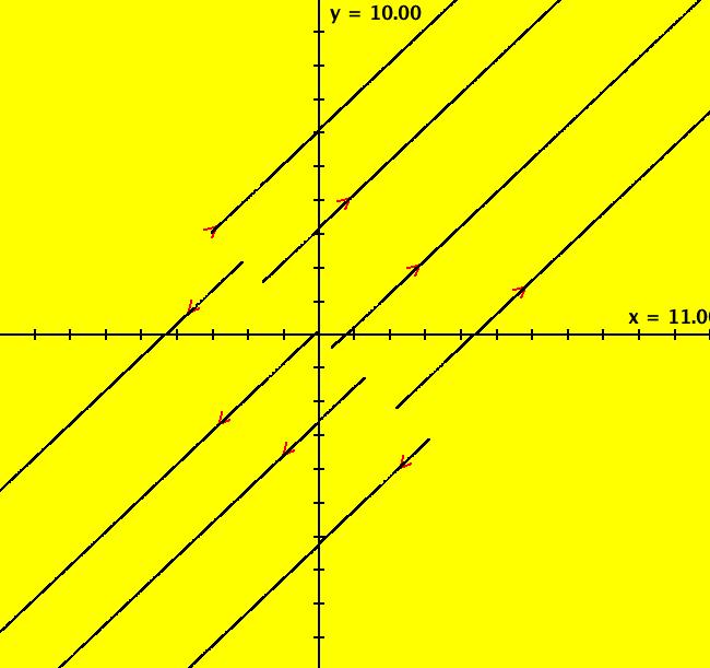
View/Sys/Gal: IMap "Fibonacci sequence as an IMap" in "OdeFactoryExs." The Fibonacci sequence is defined by the recursive function f(0) = 1, f(1) = 1, f(n+2) = f(n+1)+f(n), for int n > 0, which corresponds to the 2nd order ode in normal form given by y'' = y'+y with ICs (y(0),y'(0)) = (1,1) which in turn corresponds to the vector field V = (y,x+y). The vector field, when viewed as an IMap, with seed (x,y) = (1,1), gives the Fibonacci sequence in the 3D/(t,x) IMap view: t = 0, 1, 2, 3, 4, 5, 6 ... x = 1, 1, 2, 3, 5, 8, 13 ... Image 1: IMap 3D/(t,x) view. See: recursive functions.
|
|
View/Sys/Gal: Ode "IDE Labs/Tools, dx/dt=y, dy/dt=-d*x+r*y" in "OdeFactoryExs." This system of odes is defined by the equations: dx/dt = y, dy/dt = -d*x+r*y in the (t,x,y) coordinate system. The 1st order 2D system corresponds to the 2nd order ode y'' = -d*y+r*y' in the (x,y,y') coordinate system. Parameters are: r = -1.00; d = 2.00; The coefficient matrix is: [ 0 1] [-d r] so the r = trace and the d = determinant, or tr and det for short. The eigenvalues of the coefficient matrix are: (tr+sqrt(tr^2-4*det))/2 and (tr-sqrt(tr^2-4*det))/2 The form of the solution curves change as the point (tr,det) crosses the following three curves in the (tr,det) plane. The parabola through (0,0) opening upward, det = tr^2/4, the positive vertical axis, tr = 0, det >= 0, and the horizontal axis, det = 0. Note that tr = -1, det = 2 gives a cw spiral "in" and tr = -1, det = -2 gives a saddle node. -----> Check these results in OdeFactory by opening the control parameters controller and setting d = -2.
-----> Find the separatrices in the saddle node case using OdeFactory. Image 1: Ode view with tr = -1, det = 2.
|
|
View/Sys/Gal: EMap "IDE Labs/Tools, dx/dt=y, dy/dt=-d*x+r*y, EMapCT9" in "OdeFactoryExs." This iteration is defined by: x <- y, y <- -d*x+r*y. Parameters are: r = -1.00; d = 2.00; EMap CT: 9 Image 1: EMap view. Another fractal.
|
|
View/Sys/Gal: IMap "Lissajou figures" in "OdeFactoryExs." This system of odes is defined by the equations: dx/dt = a*cos(a*t+b), dy/dt = c*cos(c*t) Parameters are: a = 1.00; b = 1.00; c = 3.10; You can get interesting IMaps for this system. Image 1: Three distinct Ode trajectories. Get into the IMap view. Image 2: The three corresponding IMap orbits are on a single attractor. In the IMap view, click a bit in the graphics area to generate more rectangular figures (click the "Center" button to refresh the colors). Adjust the parameters.
|
|
View/Sys/Gal: IMap "Lissajou figures, IMap variation" in "OdeFactoryExs." Play with the parameters. A Math Question: where does the big rectangle centered at (0,0) come from in the IMap view? Is there just one big rectangle (hint: watch the colors change). Hint: delete all but one seed then click Flow. Image 1: IMap view.
|
|
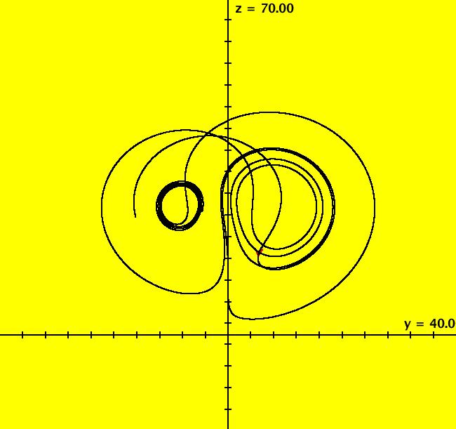
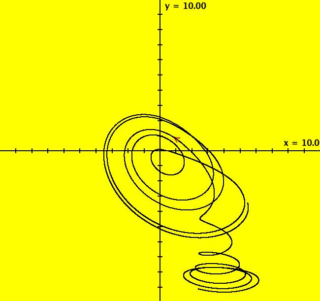
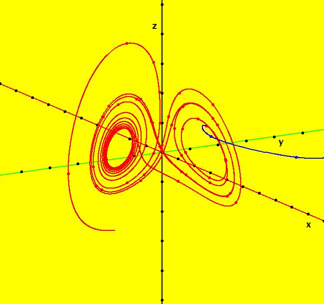
View/Sys/Gal: Ode "Lorenz attractor" in "OdeFactoryExs." This system of odes is defined by the equations: dx/dt = s*(y-x), dy/dt = x*(p-z)-y, dz/dt = x*y-b*z Parameters are: p=28; s=10; b=2.66666 Image 1: The Ode (y,z) view, with a solution started at (x,y,z) = (0,5.3,16.3). Extend the solution in +t five times. Click Flow, set dots = 0, speed = .5, duration = 40 and start the flow. Next set dots = 50 and restart the flow, notice how all dots get drawn into the attractor. Switch to -t and start the flow again. Try various values of the control parameters. See:
|
|
View/Sys/Gal: Ode "Mathematica book, p. 6, PMap ex" in "OdeFactoryExs." See: MATHEMATICA Book. This system of odes is defined by the equations: dx/dt = y, dy/dt = -x^3+sin(t) in the (t,x,y) coordinate system. The 1st order 2D system corresponds to the 2nd order ode y'' = -y^3+sin(x) in the (x,y,y') coordinate system. Image 1: Ode view. A single trajectory has been started at: (x,y) = (.74,.545455). Click on the arrowhead to open a trajectory controller then get into the 3D/(x,y) view and click on the +t button in the trajectory controller to watch the PMap (Poincare map) being generated as a sequence of black dots. For more information on the Poincare map, see: Poincare map. NOTE: This is a 2D nonautonomous system but it can be written as a 3D autonomous system by setting z = t and adding the equation dz/dt = 1.
|
|
View/Sys/Gal: EMap "Mathematica book, p. 6, PMap ex, 2D EMapCT5 variation" in "OdeFactoryExs." This system of odes is defined by the equations: dx/dt = y, dy/dt = -c*x^3+sin(t) in the (t,x,y) coordinate system. The 1st order 2D system corresponds to the 2nd order ode y'' = -c*y^3+sin(x) in the (x,y,y') coordinate system. Parameters are: c = .76; The parameter c was added to the system to get an interesting EMap. ICs for the trajectory in the Ode view are: (t,x,y) = (0,.74,.545454) OdeFactory will draw a EMap for nonautonomous 2D systems. Every nonautonomous 2D system can be rewritten as an autonomous 3D system by replacing t by z in the 2D system and adding the third equation dz/dt = 1. Image 1: Ode view. Image 2: IMap view in R2+. Image 3: EMap view.
|
|
View/Sys/Gal: Ode "Mathematica book, p. 6, PMap ex, 3D version" in "OdeFactoryExs." This system of odes is defined by the equations: dx/dt = y, dy/dt = -c*x^3+sin(z), dz/dt = 1 Parameters are: c = .76; ICs for the trajectory in the (x,y) view are: (t,x,y,z) = (0,.74,.545455,0). Image 1: Ode 3D/(t,x,y) view.
|
|
View/Sys/Gal: Ode "Mattuck Lect 31, y''=-k*sin(y)-c*y'" in "OdeFactoryExs." This system of odes is defined by the equations: dx/dt = y, dy/dt = -k*sin(x)-c*y in the (t,x,y) coordinate system. The 1st order 2D system corresponds to the 2nd order ode y'' = -k*sin(y)-c*y' in the (x,y,y') coordinate system. Parameters are: k = 2.00; c = 1.00; See Mattuck Lect 31 It is a good lecture. You should view the entire lecture when you have time. -----> Also, bring up p. 129 of the "MIT 18.03 Course Notes" to read about the theory. The easy way to enter the ode (starting with the "F=ma" form) into OdeFactory is to replace the angle theta by "y" and use the "y(x)" normal form of the 2nd order ode: y''+k*sin(x)+c*y = 0 The 1st order system of odes is then defined by the equations: dx/dt = y, dy/dt = -k*sin(x)-c*y in the (t,x,y) coordinate system. Parameters are: k = 2.00; c = 1.00; "x" is now the angular position of the pendulum and "y" is the angular velocity. ICs (x,y) = (pi/2,0) corresponds to the pendulum starting from rest at 90 degrees to the right of the bottom position. Image 1: Ode view. A trajectory with ICs (pi/2,0). The Mattuck video is 47 minutes long. He begins by deriving the equations of motion from the basic Physics. His goal is to sketch representative solution curves by hand. The algorithm used by Mattuck is: (1) find the fixed points of the system (2) linearize the system at the fixed points by evaluating the Jacobian matrix at the fixed points then find the eigenvalues and eigenvectors of the linearized system at each fixed point (3) extend the phase curves near the fixed points (by a "continuity" argument) to the rest of the phase plane We can implement the algorithm using WA and OdeFactory as follows. -----> (1) to find the fixed points, drop 0 = y, 0 = -2*sin(x)-y into WA Of course the location of the fixed points is obvious in this example but WA can just as easily be applied to cases where the fixed points would be very hard, if not impossible, to find by hand. -----> (2) next drop evaluate D[{y,-2*sin(x)-y},{{x,y}}] at x=0, y=0 into WA to evaluate the Jacobian at x=y=0 then evaluate the Jacobian matrix again at x=pi, y=0 (WA knows about "pi") -----> (3) finally use OdeFactory to draw some phase curves Actually we can do a bit better here. We can skip step (2) and instead generate separatrices at the points (x,y) = (pi,0) and (x,y) = (-pi,0). -----> In OdeFactory, we can also: - adjust the values of k and c to see what happens - turn the Flow and/or Vector field on/off (try the colored vector field) - look at the 3D view of the system Image 2: 3D view.
|
|
View/Sys/Gal: EMap "Mattuck Lect 31, y''=-k*sin(y)-c*y' EMapCT2 view" in "OdeFactoryExs." This iteration is defined by: x <- y, y <- -k*sin(x)-c*y. Parameters are: k = 9.400; c = .890; EMap CT: 2 Image 1: EMap view.
|
|
View/Sys/Gal: Ode "OdeFactory syntax demo" in "OdeFactoryExs." This example is a demo of the syntax that can be used to enter odes, parameters and user defined functions in OdeFactory. This is a really nasty system of odes. This system of odes is defined by the equations: dx/dt = x*sin(x+pi*y-t), dy/dt = a*x^2/Q-b*P Parameters are: a = 1.5; b=-2 Functions are: P = x*y; Q = sqrt(a*x+y/b) Try to start a solution at about (-1,1) to see what happens. Notice that nothing happens. The Q function is not defined at (-1,1) since sqrt has a negative argument at (-1,1). OdeFactory traps for such errors and keeps running.
|
|
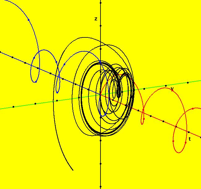
View/Sys/Gal: Ode "R2+ and 3D views of system (-x,y)" in "OdeFactoryExs." This system of odes is defined by the equations: dx/dt = -x, dy/dt = y. Image 1: R2 view. Image 2: R+ view. The R2+ view of this system is easy enough to understand but the 3D views are much harder to envision. Try the R2+ view then return to the R2 view and get into the 3D view. Image 3: 3D/(t,x,y) view. To better understand the 3D view, return to the 2D view, clear the trajectories then start a single trajectory at (t,x,y) = (0,-1,.1). Next get back into the 3D/(t,x,y) view. The red axis is the +t-axis, the blue axis is the -t-axis, the green axis is the x-axis and the black axis is the y-axis. The black curve is the trajectory in the (x,y) plane (the phase space) and the red-blue curve is the solution curve in (t,x,y) (the extended-phase space). The trajectory (black curve) is the projection of the solution curve (red-blue curve) onto the (x,y) plane. The red part of the solution curve is the +t part and the blue part is the -t part. In the 3D/(t,x,y) view, it may look like the curve starting at (0,-1,.1) crosses the (t,y) plane but it does not. You can check this out by looking down the y-axis toward (0,0,0). To do this, select the 3D/(t,x) view. Try to guess what the 3D/(t,y) view should look like, then check it out.
|
|
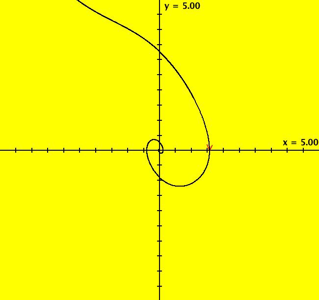
View/Sys/Gal: Ode "Riccati equation" in "OdeFactoryExs." This ode is defined by the equation: dx/dt = (2*cos(t)^2-sin(t)^2+x^2)/(2*cos(t)). This is a Riccati equation of the form: dy/dt = P(x)+Q(x)*y+R(x)*y^2 where P(x) = cos(x), Q(x) = -sin(x)^2/(2*cos(x)) and R(x) = 1/(2*cos(x)). To find the particular solution for y(0) = -1, drop y' = (2*cos(x)^2-sin(x)^2+y^2)/(2*cos(x)), y(0)=-1 into WA to get y(x) = ((1-2 i)+6 e^(2 i x)+(1+2 i) e^(4 i x))/((-4-2 i) e^(i x)-(4-2 i) e^(3 i x)) To find y(x) in real form, drop simplify ((1-2 i)+6 e^(2 i x)+(1+2 i) e^(4 i x))/((-4-2 i) e^(i x)-(4-2 i) e^(3 i x)) into WA to get sin(x)-2/(2 cos(x)+sin(x)) so y(x) = sin(x)-2/(2 cos(x)+sin(x)) and y(0) = -1, as it should. To see how to solve this problem by hand, see the second example on Web page Riccati equation. Image 1: A sample trajectory.
|
|
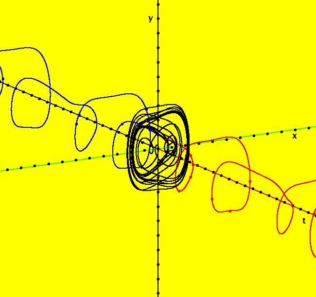
View/Sys/Gal: Ode "Rossler attractor" in "OdeFactoryExs." This system of odes is defined by the equations: dx/dt = -y-z, dy/dt = x+a*y, dz/dt = b+z*(x-c) Parameters are: a=.432; b = 2; c = 4 Starting point is: t = 0, x = 1.16, y ~ 1.46, z = 0. See: Rossler attractor Image 1: A chaotic trajectory in the 3D/(t,x,y) view. Is the system chaotic for all values of the control parameters? Click on "Adj Ctrl Params..." and vary the control parameters to answer this question.
|
|
View/Sys/Gal: Ode "Rossler attractor again, different ICs" in "OdeFactoryExs." This system of odes is defined by the equations: dx/dt = -y-z, dy/dt = x+a*y, dz/dt = b+z*(x-c) Parameters are: a=.432; b = 2; c = 4 Starting point is: t = 0, x = .92, y = .87, z = 1. Image 1: A chaotic trajectory. Click on the arrowhead and extend the trajectory.
|
|
View/Sys/Gal: Ode "Sprott case C, simple chaotic flow" in "OdeFactoryExs." This system of odes is defined by the equations: dx/dt = y*z, dy/dt = x-y, dz/dt = 1-x*x Solution starts at x = y = z = 1 in the (y,z) view. Image 1: The (x,y,z) view shows the trajectory in the 3D phase space. The red part is +t, the blue part is -t. To see an animation, select the (y,z) view and click the "Flow..." button. For more details, and further examples of chaotic flows, see: Sprott. Add some control parameters and adjust them to see what happens.
|
|
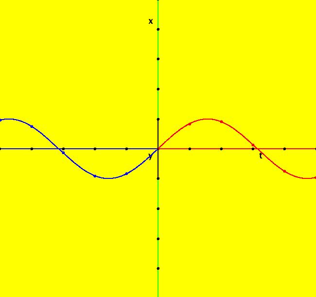
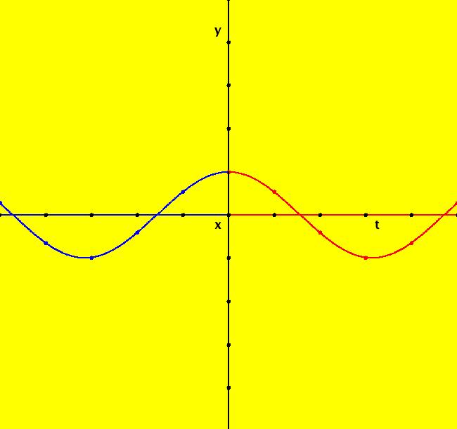
View/Sys/Gal: Ode "definition of sin(t) and cos(t)" in "OdeFactoryExs." This system of odes is defined by the equations: dx/dt = y, dy/dt = -x. In the 3D view, see the (t,x) projection and the (t,y) projection. Image 1: 3D/(t,x). Image 2: 3D/(t,y). Try Flow. Try V On. Try the IMap 3D/(x,y) view.
|
|
View/Sys/Gal: Ode "definition of sinh(t) and cosh(t)" in "OdeFactoryExs." This system of odes is defined by the equations: dx/dt = y, dy/dt = x. In the 3D view, x(t) = sinh(t) and y(t) = cosh(t). Image 1: 3D/(t,x), x(t) = sinh(t). Image 2: 3D/(t,y), y(t) = cosh(t). Try the 3D/(x,y) IMap view.
|
|
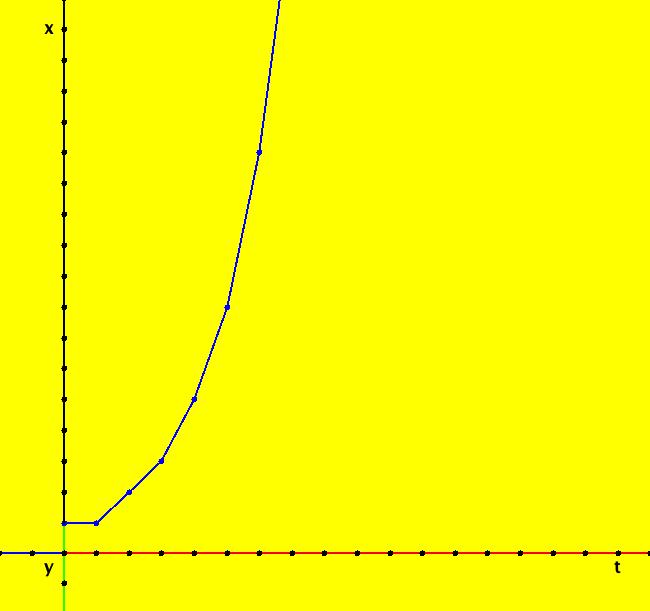
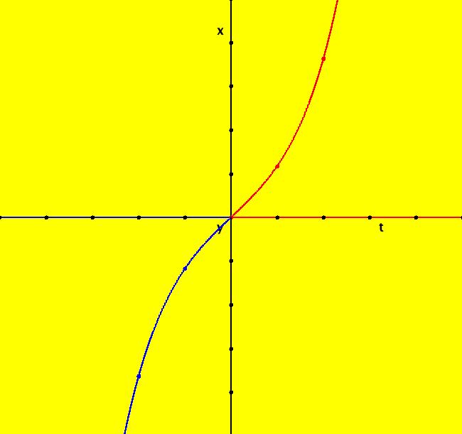
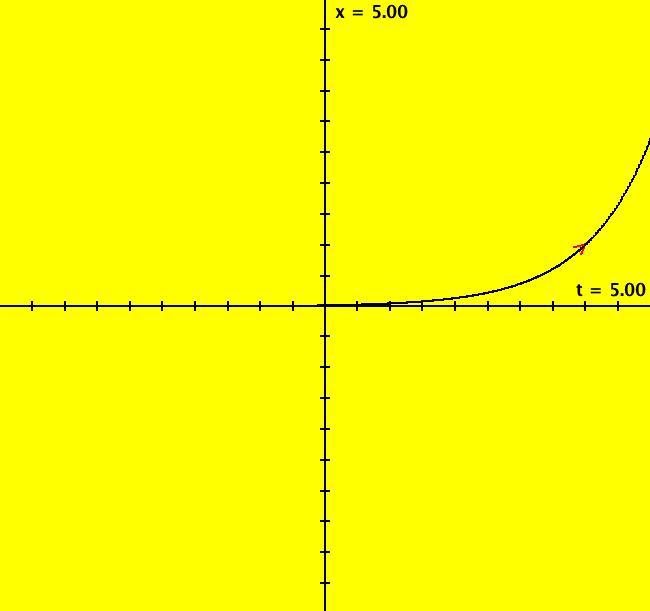
View/Sys/Gal: Ode "definition of x(t) = e^t" in "OdeFactoryExs." This ode is defined by the equation: dx/dt = x. Compute e by starting a solution at (4,1), closing the border then clicking on the arrowhead. Explain the result. Image 1: Ode trajectory with ICs (4,1).
|
|
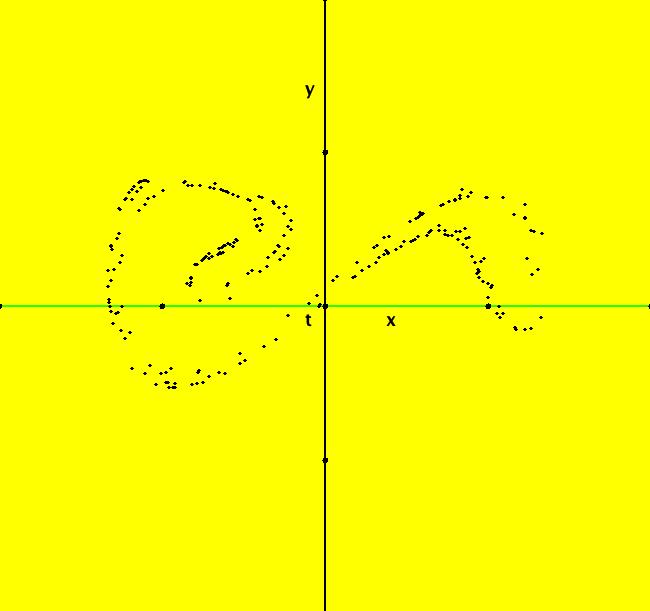
View/Sys/Gal: Ode "driven pendulum, PMap ex" in "OdeFactoryExs." This example is from Guckenheimer and Holmes, "Nonlinear Oscillations, Dynamical Systems, and Bifurcations of Vector Fields," p. 29. This is a pendulum with a periodically excited support (G&H eqn 1.5.23a). The system of odes is defined by the equations: dx/dt = y, dy/dt = -(a^2+b*cos(t))*sin(x). Trajectories near (x,y) = (0,0) are red in OdeFactory because |v| is close to 0. Image 1: Ode view with ICs: (0.200000,0.141414), (0.168000,0.068687), (0.080000,0.030303), (0.037807,0.009619). Select t, in addition to x and y, to get to the 3D view, click in the viewing area to open the 3D controller and select the 3D/(x,y) subview to see the Poincare map (PMap). Image 2: 3D/(x,y) PMap view. Dotted lines indicate that the trajectories are probably chaotic.
|
|
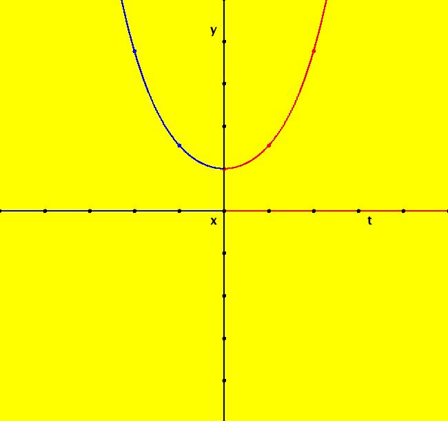
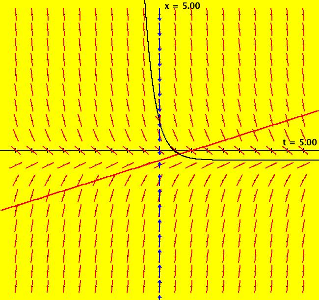
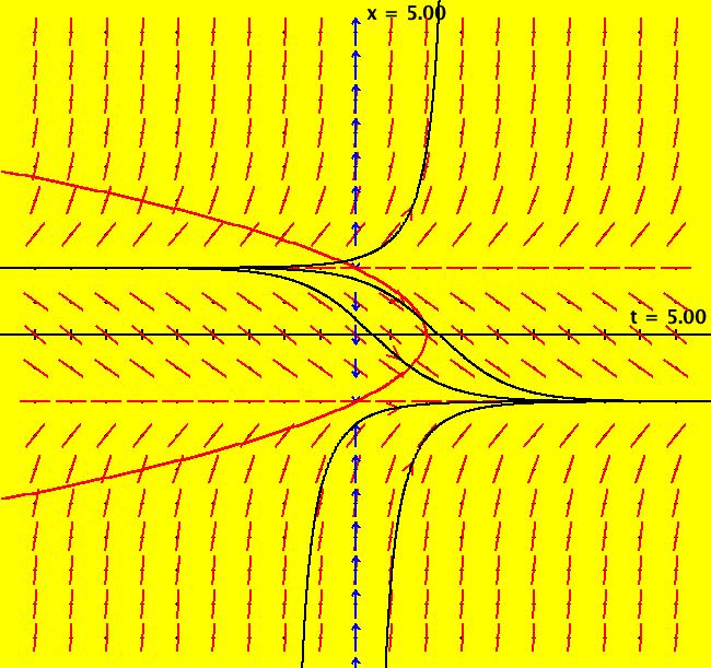
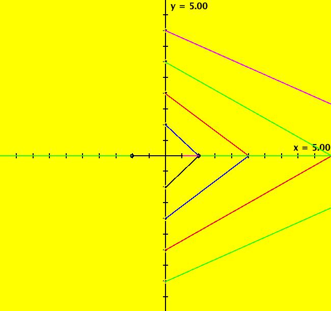
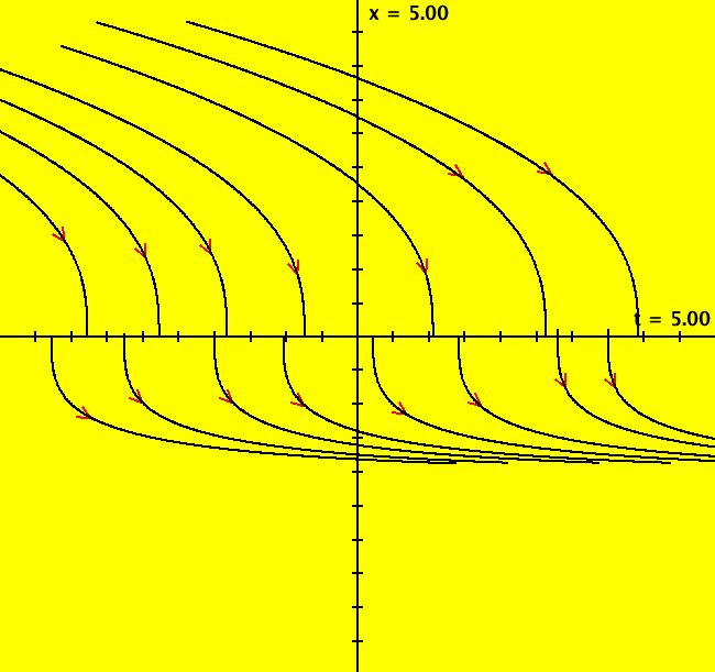
View/Sys/Gal: Ode "dx/dt = -3*x-1, aka y' = -3*y-1" in "OdeFactoryExs." This ode is defined by the equation: dx/dt = -3*x-1. If you drop the ode into the entry field of WolframAlpha (WA for short), you get the solution: x(t) = c_1 e^(-3 t)-1/3 NOTE: you can just use copy-paste to "drop" equations, or any WA expressions, from any OdeFactory window into WA. For a 1D system, the x axis is the phase space. The (t,x) plain is the extended phase space. The blue arrows on the x axis show the direction of the motion in the phase space. The red curve is the line "y(x) = -3*x-1," where "+y" is the -t axis. The fixed points of the system are the zeros of the driving function, -3*x-1. They are also the asymptotic values of the solution curves. If you click on the arrow head you get: p(15.0299999999997240) = (-0.3333333333333324) Image 1: Slope field with a solution curve.
|
|
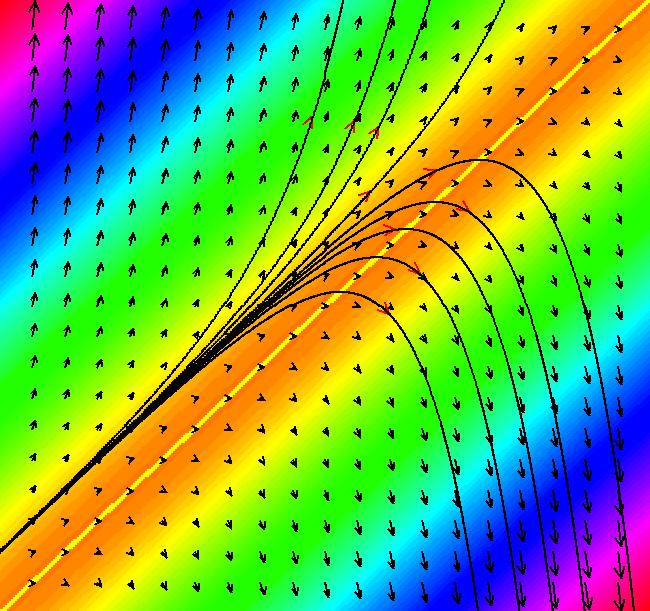
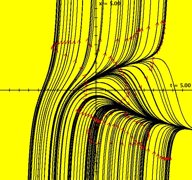
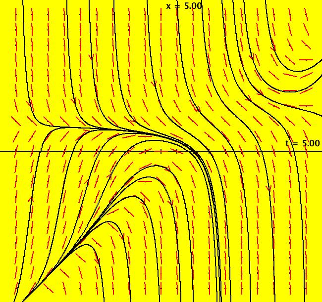
View/Sys/Gal: Ode "dx/dt = 1, dy/dt = y-x from dx/dt = x-t" in "OdeFactoryExs." This is the 2D autonomous version of the 1D nonautonomous ode: dx/dt = x-t or y' = y-x. y' = dy/dx = (dy/dt)/(dx/dt) = (y-x)/1 so dx/dt = 1, dy/dt = y-x The slope of the vector field for this 2D system is the slope of the slope field for the corresponding 1D system. Note: going from a 1D nonautonomous system to the corresponding 2D system always gives an autonomous system. Note: going from a 2D system to the corresponding 1D system is sometimes useful since lower order odes are often easier to solve by hand. Try WA on both the 2D system and the 1D system. Image 1: Colored vector field and trajectories of the 2D autonomous version of the 1D nonautonomous system.
|
|
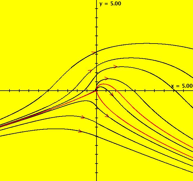
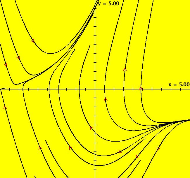
View/Sys/Gal: Ode "dx/dt = abs(x)+y^2, dy/dt = -x+y" in "OdeFactoryExs." This system of odes is defined by the equations: dx/dt = abs(x)+y^2, dy/dt = -x+y. The red separatrix curves start at: (x,y) = (-.001,.001) and (.001,-.001). Image 1: The Ode R2 view. Image 2: The Ode R2+ view.
|
|
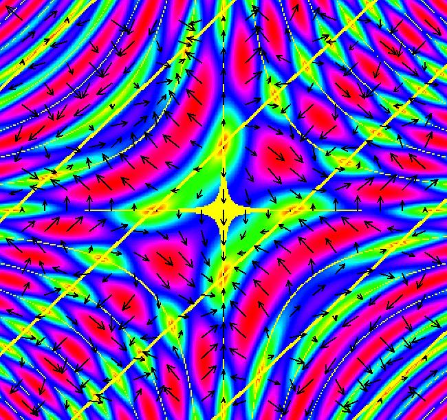
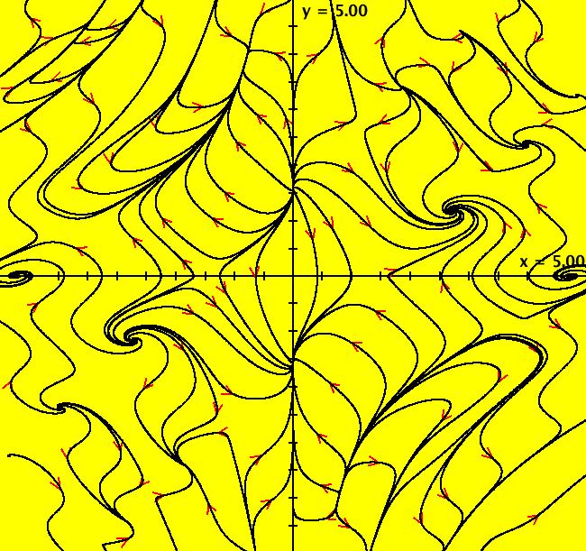
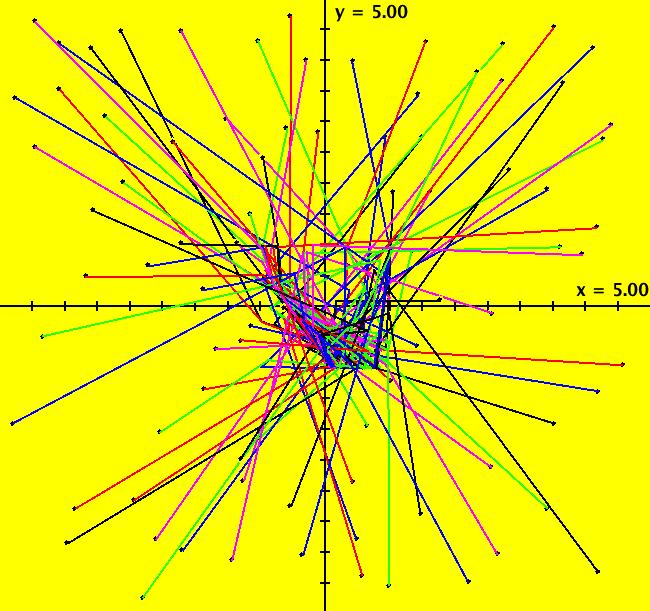
View/Sys/Gal: IMap "dx/dt = sin(x*y), dy/dt = -cos(x-y)" in "OdeFactoryExs." This system of odes is defined by the equations: dx/dt = sin(x*y), dy/dt = -cos(x-y) Image 1: The colored vector field with yellow isoclines. Image 2: Ode view with trajectories. Image 3: The IMap view. All orbits go to the fixed point (0.000000,-0.739085). Show that as an Ode the system has an infinite number of: spiral-in points, spiral-out points, saddle points, source nodes and sink nodes but no fixed points at infinity.
|
|
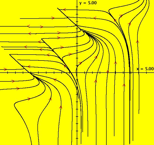
View/Sys/Gal: Ode "dx/dt = sin(x+y), dy/dt = e^(x-y)" in "OdeFactoryExs." This system of odes is defined by the equations: dx/dt = sin(x+y), dy/dt = e^(x-y) Image 1: Ode view.
|
|
View/Sys/Gal: Ode "dx/dt = sin(y), dy/dt = cos(x)" in "OdeFactoryExs." This system of odes is defined by the equations: dx/dt = sin(y), dy/dt = cos(x). Image 1: Some trajectories in the Ode view with the vector field on. Add more trajectories. Try the IMap view.
|
|
View/Sys/Gal: EMap "dx/dt = x*y+p, dy/dt = x+y+q, p = -.050; q = .800; as EMapCT1" in "OdeFactoryExs." This iteration is defined by: x <- x*y+p, y <- x+y+q. Parameters are: p = -.050; q = .800; EMap CT: 1 Image 1: EMap view. Try some different color tables and parameter values.
|
|
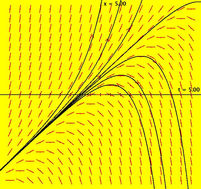
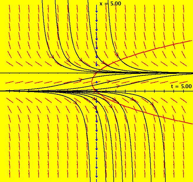
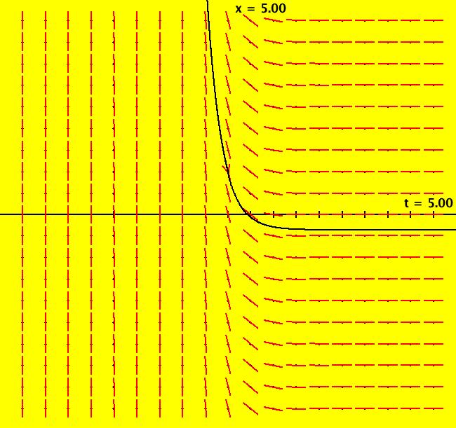
View/Sys/Gal: Ode "dx/dt = x-t" in "OdeFactoryExs." This ode is defined by the equation: dx/dt = x-t in the (t,x) coordinate system. The 1st order 1D system corresponds to the 1st order ode y' = y-x in the (x,y) coordinate system. Image 1: Ode view with the slope field on. Try the IMap view.
|
|
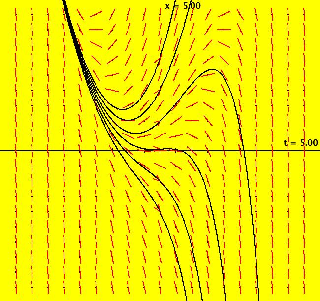
View/Sys/Gal: Ode "dx/dt = x-t^2" in "OdeFactoryExs." This ode is defined by the equation: dx/dt = x-t^2 in the (t,x) coordinate system. The 1st order 1D system corresponds to the 1st order ode y' = y-x^2 in the (x,y) coordinate system. Use WA to find the solution: x(t) = c_1 e^t+t^2+2 t+2 Image 1: Ode view with the slope field on.
|
|
View/Sys/Gal: EMap "dx/dt = x^2+y, dy/dt = x-y^2" in "OdeFactoryExs." This system of odes is defined by the equations: dx/dt = x^2+y, dy/dt = x-y^2 Image 1: The Ode R2+ view. Image 2: The EMap looks like a bird. Add some parameters and play with the system.
|
|
View/Sys/Gal: EMap "dx/dt = x^2+y, dy/dt = x-y^2 w/params EMapCT3" in "OdeFactoryExs." This iteration is defined by: x <- a*x^2+y, y <- x-b*y^2. Parameters are: a = .64; b = 1.00; EMap CT: 3 Image 1: Ode view. Image 2: IMap view. Image 3: EMap view.
|
|
View/Sys/Gal: Ode "dx/dt = x^2-r^2" in "OdeFactoryExs." This ode is defined by the equation: dx/dt = x^2-r^2 in the (t,x) coordinate system. The 1st order 1D system corresponds to the 1st order ode y' = y^2-r^2 in the (x,y) coordinate system. Parameters are: r=1 From WA the solution is: x(t) = -r tanh(r t-c_1 r) Image 1: Ode view. Vary r. For this system, the IMap is much more interesting mathematically than the Ode - as will be seen in the next example.
|
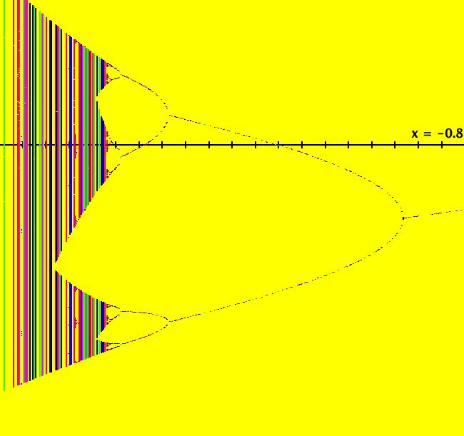
| View/Sys/Gal: IMap "dx/dt = x^2-r^2's IMap0001 bifurcation diagram" in "OdeFactoryExs." This iteration is defined by: x <- x, y <- y^2-x^2. It is the bifurcation diagram for the 1D one parameter Ode: dx/dt = x^2-r^2 when the Ode is viewed in the IMap view. If we think of the x axis for the 2D IMap as the parameter "r" in the 1D IMap: x <- x^2-r^2 the 1D IMap has orbits of period 1, 2, 4, 8, ... going to chaotic.
Image 1: The bifurcation diagram for the IMap: x <- x^2-r^2.
|
|
View/Sys/Gal: Ode "dx/dt = x^2-t" in "OdeFactoryExs." This ode is defined by the equation: dx/dt = x^2-t in the (t,x) coordinate system. The 1st order 1D system corresponds to the 1st order ode y' = y^2-x in the (x,y) coordinate system. Use WA to find the solution: x(t) = (i t^(3/2) (-c_1 J_(-4/3)(2/3 i t^(3/2))+c_1 J_(2/3)(2/3 i t^(3/2))-2 J_(-2/3)(2/3 i t^(3/2)))-c_1 J_(-1/3)(2/3 i t^(3/2)))/(2 t (c_1 J_(-1/3)(2/3 i t^(3/2))+J_(1/3)(2/3 i t^(3/2)))) Image 1: Ode view.
|
|
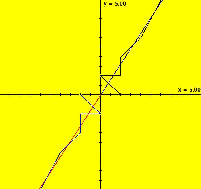
View/Sys/Gal: IMap "dx/dt = y, dy/dt = x+y" in "OdeFactoryExs." This system of odes is defined by the equations: dx/dt = y, dy/dt = x+y in the (t,x,y) coordinate system. The 1st order 2D system corresponds to the 2nd order ode y'' = y+y' in the (x,y,y') coordinate system. WA, applied to the system, gives solutions: x(t) = 1/10 c_1 (e^(-1/2 (sqrt(5)-1) t) (sqrt(5)-(sqrt(5)-5) e^(sqrt(5) t))+5 e^(1/2 (1-sqrt(5)) t))-(c_2 (e^(1/2 (1-sqrt(5)) t)-e^(1/2 (1+sqrt(5)) t)))/sqrt(5) y(t) = 1/10 c_2 (e^(-1/2 (sqrt(5)-1) t) ((5+sqrt(5)) e^(sqrt(5) t)-sqrt(5))+5 e^(1/2 (1-sqrt(5)) t))-(c_1 (e^(1/2 (1-sqrt(5)) t)-e^(1/2 (1+sqrt(5)) t)))/sqrt(5) WA applied to y'' = y+y' gives: y(x) = c_1 e^(-1/2 (sqrt(5)-1) x)+c_2 e^(1/2 (1+sqrt(5)) x) WA applied to {x,y}=MatrixExp[{{0,1},{1,1}}t].{0,1} gives: {x, y} = {-(e^(1/2 (1-sqrt(5)) t)-e^(1/2 (1+sqrt(5)) t))/sqrt(5), 1/10 (5 e^(1/2 (1-sqrt(5)) t)-sqrt(5) e^(1/2 (1-sqrt(5)) t)+5 e^(1/2 (1+sqrt(5)) t)+sqrt(5) e^(1/2 (1+sqrt(5)) t))} Apply WA to {{0,1},{1,1}} to find the eigenvectors and eigenvalues of the system. Image 1: Ode view. Image 2: IMap view.
|
|
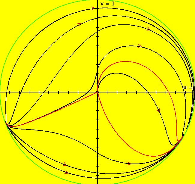
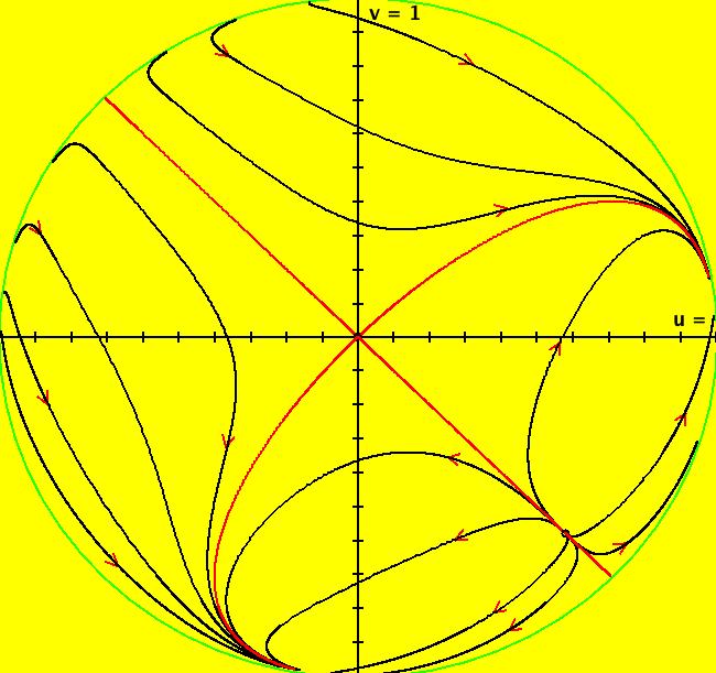
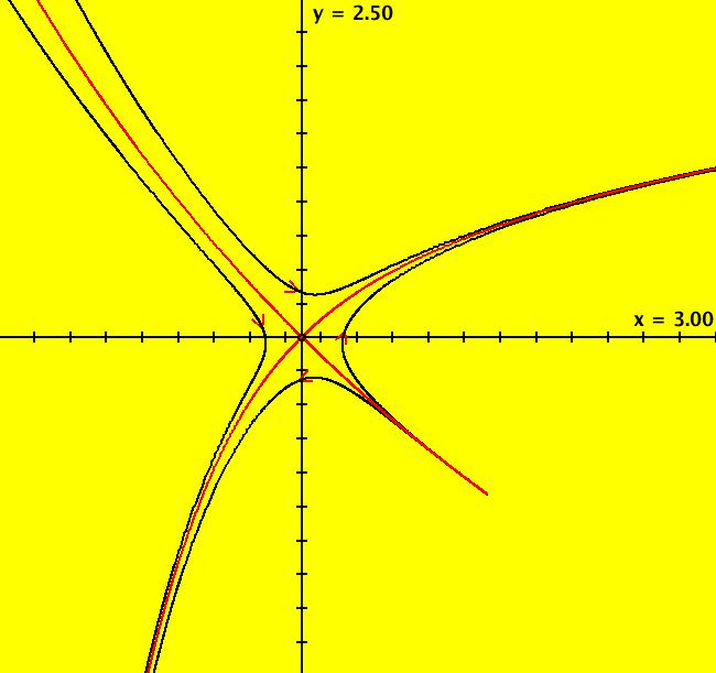
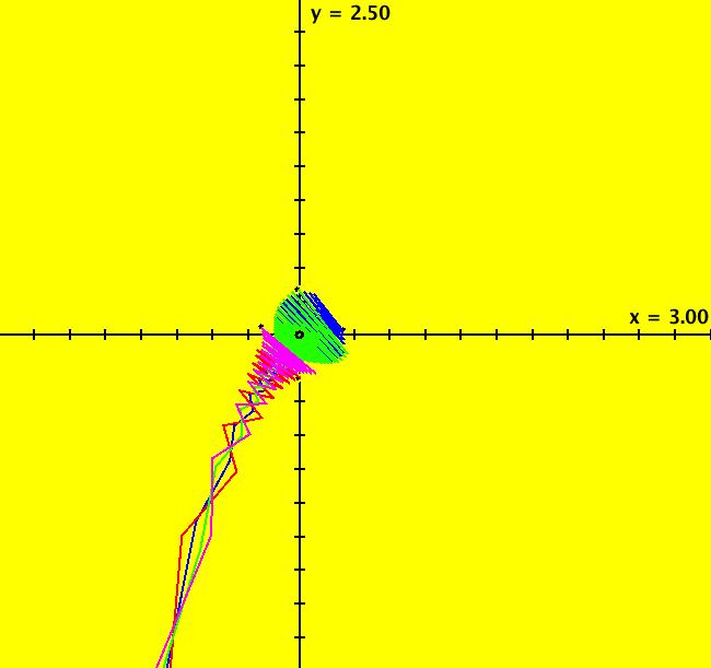
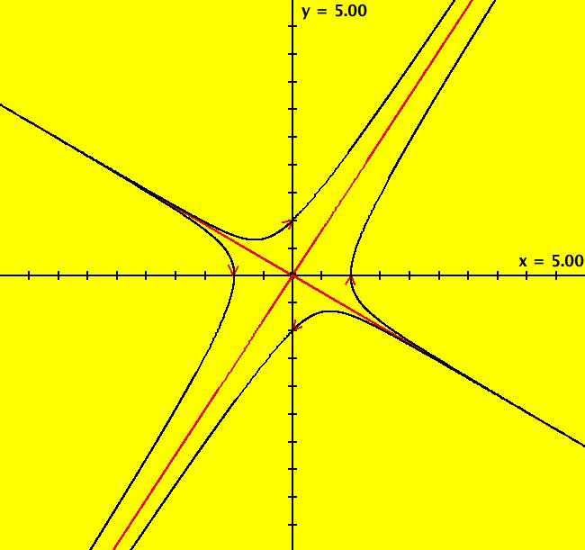
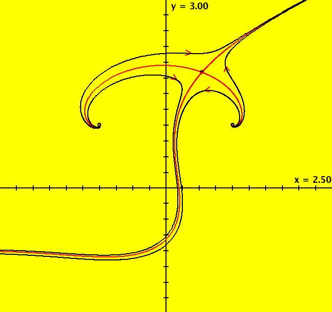
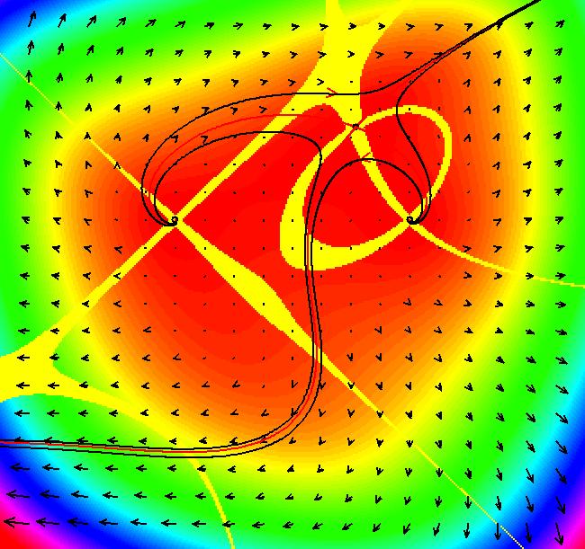
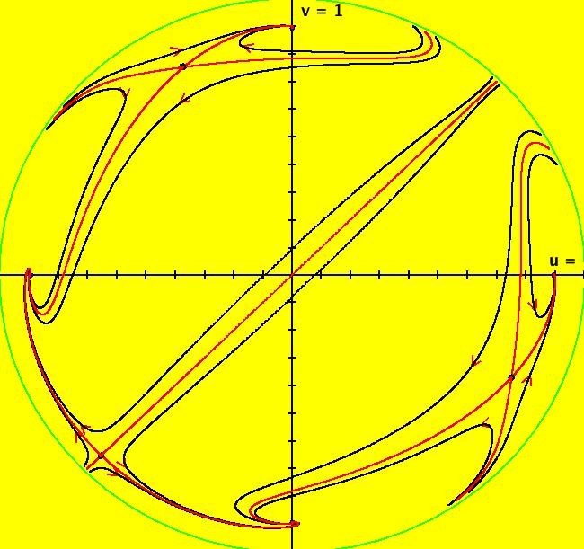
View/Sys/Gal: Ode "finding separatrices of a cubic system" in "OdeFactoryExs." This system of odes is defined by the equations: dx/dt = x*(0.5*x^2+0.5)+y*(-x+(0.5*y-1)*y+0.5), dy/dt = 0.5*x^2*y+x*(-0.5*y^2+y-0.5)+0.5*y-1 Drop: 0 = x*(0.5*x^2+0.5)+y*(-x+(0.5*y-1)*y+0.5), 0 = 0.5*x^2*y+x*(-0.5*y^2+y-0.5)+0.5*y-1 into WA to find the approximate fixed points: x = 0.543689, y = 1.83929 x = 1, y = 1 x = -1, y = 1 then start trajectories at, and near, the first fixed point. The four red curves are the separatrices. Image 1: Ode view. In OdeFactory there is graphical way to find the fixed points for a 2D autonomous system. When you turn the colored vector field on you can see the fixed points where the nullclines cross. Image 2: Ode view with colored vector field on. Where are the fixed points at infinity? Find the (u,v) coordinates on the Poincare disk (hint: try the R2+ view). Image 3: Ode R2+ view.
|
|
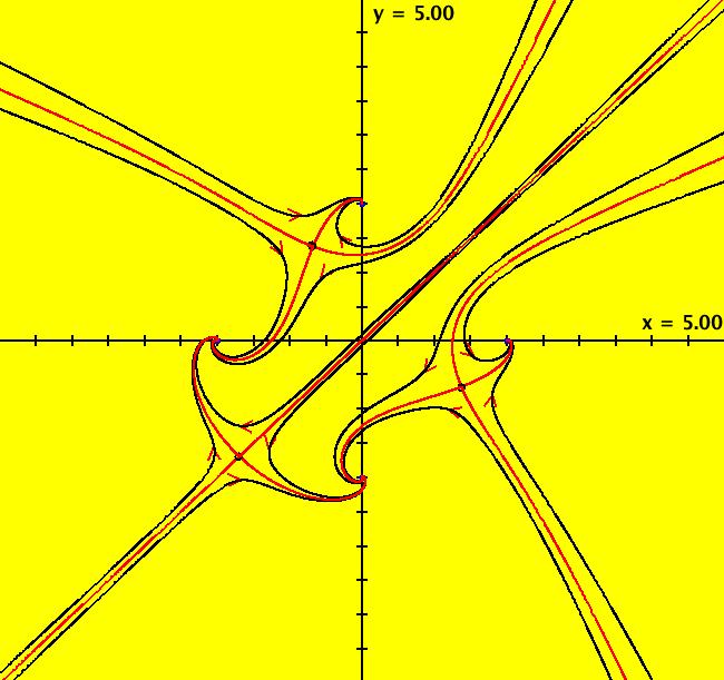
View/Sys/Gal: Ode "finding separatrices of an AGF" in "OdeFactoryExs." This AGF is generated by the lines: I[1]: x+i*y = 0, λ1 = i I[2]: (x-1)+i*(y-1) = 0, λ2 = (1-i) The degree of the RHS of the system is: 3. To find possible fixed points, turn the colored vector field on and look for small black regions where nullclines cross. The two generators are centered at (0,0) and (1,1) which are fixed points. It looks like there is a third fixed point near (-1,1). Start a trajectory near (-1,1). Turn the vector field off, center near (-1,1) and zoom in. Start trajectories near (-1,1) until you find two red trajectories, close together that look like straight lines. Delete extraneous trajectories, center at (0,0), zoom out and switch to the R2+ view. Add representative trajectories in regions defined by the separatrices. Image 1: Ode R2 view. Image 2: Ode R2 view with colored vector field on. Image 3: Ode R2+ view.
|
|
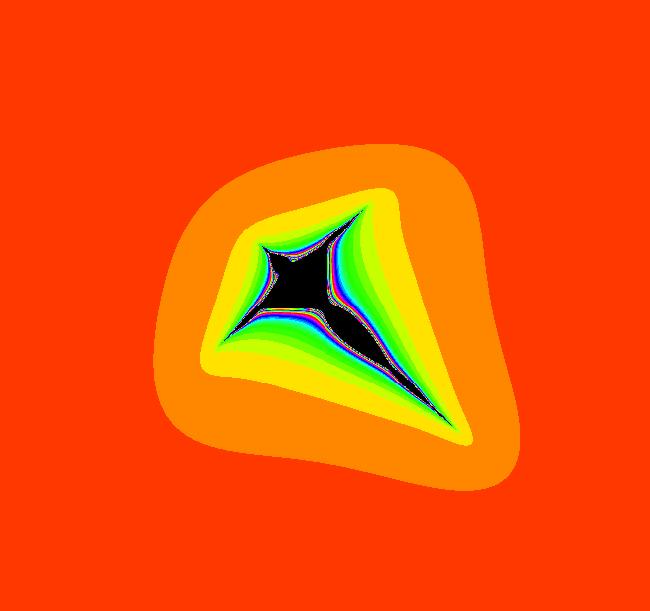
View/Sys/Gal: EMap "finding the EMap for an AGF" in "OdeFactoryExs." This AGF is generated by the lines: I[1]: (x-0.04)+i*y = 0, λ1 = 1.2*i I[2]: (x-1)+i*(y-1) = 0, λ2 = (1-i) The degree of the RHS of the system is: 3. The system is a slight modification of the previous example. The location of I[1] has been shifted right by .04 and the eigenvalue has been scaled by 1.2 to get an "interesting" EMap. To adjust the EMap parameters, go back to the Ode view then shift-click on I[1], the green dot near (0,0). A slider-based parameter controller for I[1] will open. Slowly adjust some or the parameters. If you are interested in the Ode, you can toggle to the Ode view and adjust parameters to watch the flow change. You can also adjust the parameters associated with I[2] centered at (1,1). Each complex generator has 8 control parameters so the system has 16 control parameters. Image 1: EMap view.
|
|
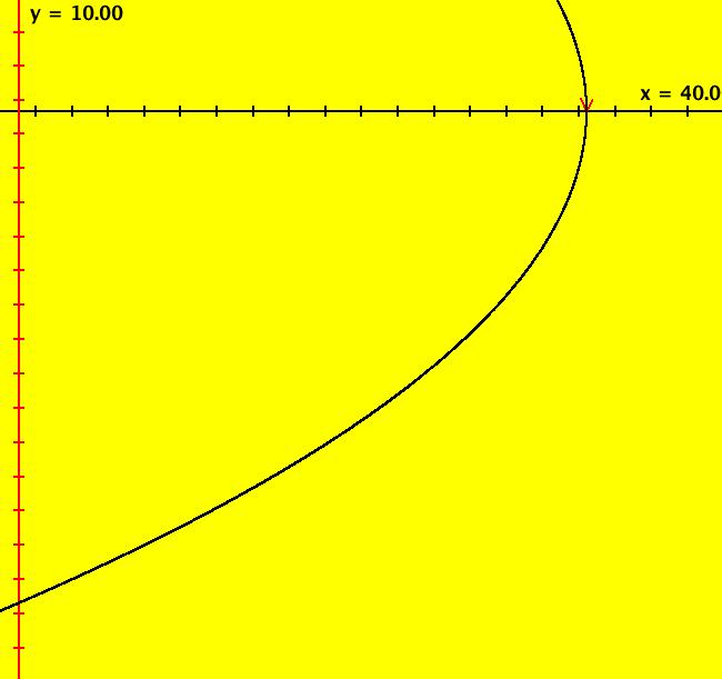
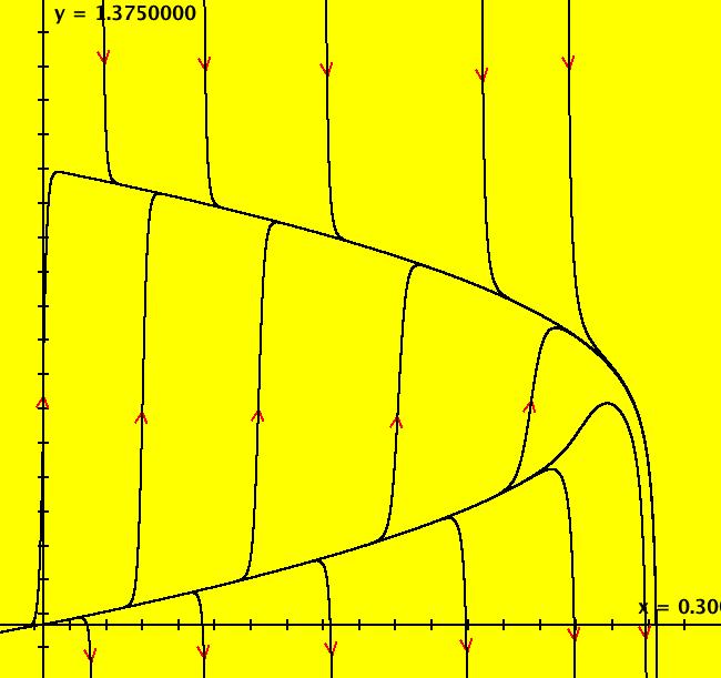
View/Sys/Gal: Ode "fireman catches baby" in "OdeFactoryExs." A building is on fire and a baby must be dropped from a 3rd floor window to a fireman on the ground. the distance between the floors is 10 feet, the windows are 3 feet above each floor and the fireman catches the baby 3 feet off the ground. How fast is the baby going, in miles/hour, when the fireman catches the baby? Let x be the vertical distance and y be the velocity so dx/dt = y and by Newton's law dy/dt = -g = -32 ft/sec/sec. Start a trajectory in the (x,y) view with ICs (t,x,y) = (0,33,0). Find y when x = 3 and convert it to miles/hour using 60 mi/hr = 88 ft/sec. To find y when x = 3, set hMin = 3, hMax = 40, vMax = 10 and vMin -50 and set the border to red. Then click on the arrowhead to get p(1.370100) = (2.965216,-43.843200). This tells you that at time = 1.370100 sec, x = 2.965216 ft and y = -43.843200 ft/sec = -29.89 mi/hr
|
|
View/Sys/Gal: Ode "four spiral sinks and three saddles" in "OdeFactoryExs." This AGF is generated by the lines: I[1]: (x-2)+i*y = 0, λ1 = (-1-i) I[2]: (x+2)+i*y = 0, λ2 = (-1+i) I[3]: x+i*(y-2) = 0, λ3 = (-1+i) I[4]: x+i*(y+2) = 0, λ4 = (-1-i) The degree of the RHS of the system is: 7. The system has 4 spiral sinks and 3 saddles. Image 1: Ode R2 view. Image 2: Ode R2+ view.
|
|
View/Sys/Gal: IMap "four spiral sinks and three saddles EMap ver" in "OdeFactoryExs." This AGF is generated by the lines: I[1]: -0.71*(x+0.67)+(0.12-0.81*i)*(y-0.01) = 0, λ1 = (0.3+0.5*i) I[2]: (x+2)+i*y = 0, λ2 = (-1+i) I[3]: x+i*(y-2) = 0, λ3 = (-1+i) I[4]: x+i*(y+2) = 0, λ4 = (-1-i) The degree of the RHS of the system is: 7. This system came from the AGF: "four spiral sinks and three saddles" by varying the defining parameters of complex line I[1] which is now located at (x,y) = (-.67,.01). I[1] was a ccw spiral in, it is now a cw spiral out. Image 1: EMap view. Image 2: Ode view. Image 3: IMap view.
|
|
View/Sys/Gal: Ode "general linear 2D system, A = {{a,b},{c,d}}" in "OdeFactoryExs." This system of odes is defined by the equations: dx/dt = a*x+b*y, dy/dt = c*x+d*y Parameters are: a=1; b=1; c=1; d=1 Image 1: Ode view with a = b = c = 1. Adjust the parameters.
|
|
View/Sys/Gal: Ode "infinite number of limit cycles?" in "OdeFactoryExs." This system of odes is defined by the equations: dx/dt = y, dy/dt = a*x+cos(x)*y. Parameters are: a = -2 Image 1: Ode view with 6 limit cycles. To find a limit cycle start a trajectory, extend it forward, save (x,y) at the +t end, delete the trajactory then start a new trajectory at (x,y). See example 9.4.2, p. 311 of Hubbard and West, "Differential Equations: A Dynamical Systems Approach." There are an infinite number of limit cycles. The result was proven in 1980 by Zhang Zhi-fen. Values of a = -1 and 1.8 give interesting EMaps if you zoom in.
|
|
View/Sys/Gal: EMap "infinite number of limit cycles? EMapCT5" in "OdeFactoryExs." This iteration is defined by: x <- y, y <- a*x+cos(x)*y. Parameters are: a = -2.000; EMap CT: 5
|
|
View/Sys/Gal: Ode "logistic equation" in "OdeFactoryExs." This ode is defined by the equation: dx/dt = x*(1-x)-h. Parameters are: h=0 For h = 0 it is just called the logistic equation and when h > 0 it is called the logistic equation with harvesting. Image 1: Ode view with S on, h = 0. Fixed points are at x = 0 and x = 1. Note that the motion is only in the +x direction between the fixed points. Increasing h brings the fixed points together and changes the nature of the solution curves (try it yourself). The parameter h is called a "bifurcation" parameter. The bifurcation curve is found by setting dx/dt = 0 to get x(h) = (1+-sqrt(1-4*h))/2, h >= 0. To draw a bifurcation curve in OdeFactory switch to the 2D system dx/dt = .001*a, dy/dt = y*(1-y)-x. Now x plays the role of the bifurcation parameter h and the bifurcation curve is y = (1+-sqrt(1-4*x))/2, x >= 0. See the next system "logistic equation w/bifurcation curve."
|
|
View/Sys/Gal: Ode "logistic equation w/bifurcation curve" in "OdeFactoryExs." This system of odes is defined by the equations: dx/dt = .001*a, dy/dt = y*(1-y)-x Parameters are: a=1 The bifurcation curve is the parabola: y = (1+-sqrt(1-4*x))/2, 0 <= x <= 1/4. It can be approximated by decreasing "a" to 0. Image 1: Approximate bifurcation curve for the 1D Ode system: dx/dt = x*(1-x)-h. Think of the x axis of this 2D system as "h" for the 1D system. You can also see the bifurcation curve by turning the colored vector field and looking for the black region. Image 2: Approximate bifurcation curve for the 1D Ode system with colored vector field on.
|
|
View/Sys/Gal: EMap "logistic equation w/bifurcation curve EMapCT7" in "OdeFactoryExs." This iteration is defined by: x <- .001*a, y <- y*(1-y)-x. Parameters are: a = 1.000; EMap CT: 7 Image 1: Another EMap Art image.
|
|
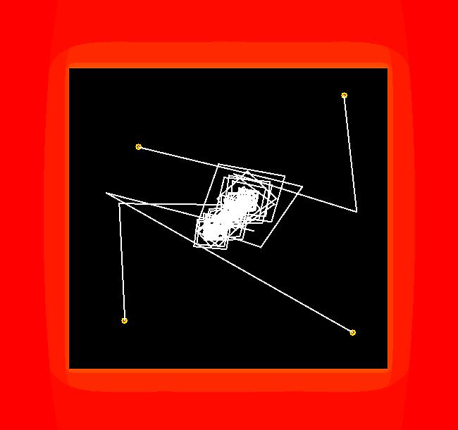
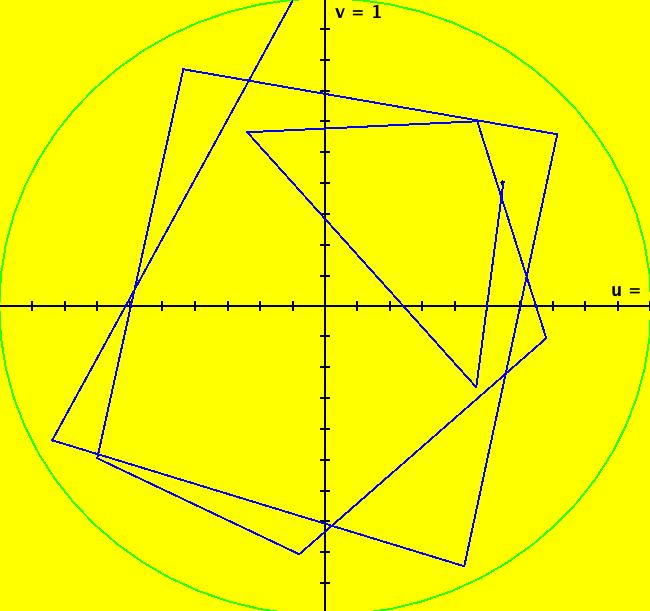
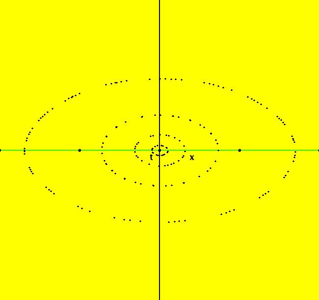
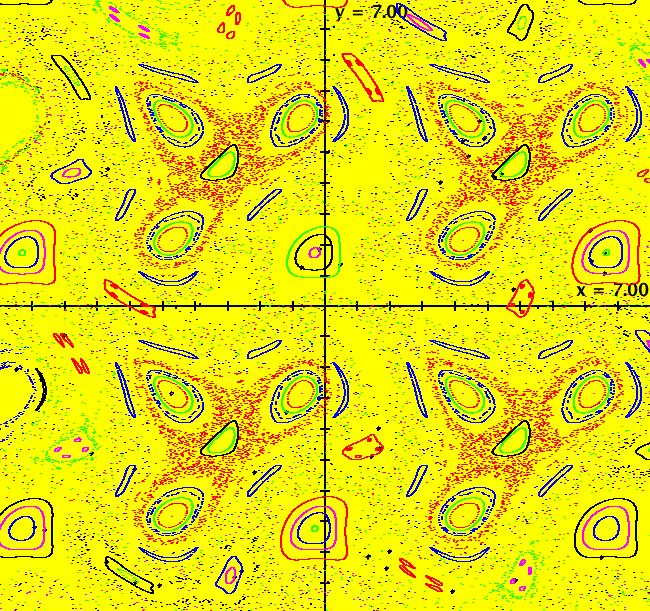
View/Sys/Gal: IMap "ode/IMap/emap, with params a and b" in "OdeFactoryExs." This iteration is defined by: x <- y-b*cos(x), y <- a-x. Parameters are: a = 1.000; b = 1.500; Wait for the image to appear. Image 1: IMap view with 39 orbits. The regular patterns are due to periodic orbits and the dust indicates chaotic orbits. Centers of regular patterns correspond to periodic orbits with small periods. Doted ellipses correspond to periodic orbits with large periods. Image 2: IMap view, after a Flow animation, with "Show 2D IMap Orbit Sequence" on shows a black dot with a white or red center which is orbit 39 at (-3.298718,-1.984467) that has period 12. Try adjusting the parameters a and b.
|
|
View/Sys/Gal: EMap "ode/IMap/emap, with params a and b EMapCT5" in "OdeFactoryExs." This iteration is defined by: x <- y-b*cos(x), y <- a-x. Parameters are: a = .700; b = 1.400; EMap CT: 5 Image 1: EMap view.
|
|
View/Sys/Gal: EMap "ode/imap/emap, with param a" in "OdeFactoryExs." This system of odes is defined by the equations: dx/dt = y-cos(x), dy/dt = a-x Parameters are: a = 1.00; ICS are: (x,y) = (5,0), (11.192366,0), (17,0). Wait for the left and right trajectories to draw. It takes a bit of time because the middle trajectory extends to about +t = 400. Image 1: Ode view. To study the middle trajectory, which is an approximate limit cycle with period 6.312, delete the other two trajectories then set vMax = 20 = -vMin, hMin = -10, hMax = 400 and center at (x,y) = (195,0). Next select the trajectory, extend the graphics area to the screen width, get into the 3D/(t,x) subview and look for repeating sets of dots on the graph of x(t). Conjecture: as an ode, this system has an infinite number of limit cycles. To see that this may be true, zoom out, clear the view then start 200 dots, at max speed, and watch them converge to +t and -t limit cycles. For a = 0, all trajectories are cycles about (0,1). The system is also interesting as a 2D iterative map. Click the "IMap" button, adjust parameter "a", add some orbits, watch what happens. Image 2: IMap view with additional orbits.. Zoom in and out to see the complexity of the 2D IMaps at both small and large scales. Try the EMap view. Image 3: EMap view. See sample gallery MapExs for several variations of this system.
|
|
View/Sys/Gal: Ode "simple pendulum" in "OdeFactoryExs." This system of odes is defined by the equations: dx/dt = y, dy/dt = -a*x in the (t,x,y) coordinate system. The 1st order 2D system corresponds to the 2nd order ode y'' = -a*y in the (x,y,y') coordinate system. Parameters are: a=1
|
|
View/Sys/Gal: EMap "simple pendulum EMapCT2" in "OdeFactoryExs." This iteration is defined by: x <- y, y <- -a*x. Parameters are: a = 1.400; EMap CT: 2
|
|
View/Sys/Gal: Ode "simplest chaotic circuit" in "OdeFactoryExs." This system of odes is defined by the equations: dx/dt = y, dy/dt = -x/3+y*(1-z^2)/2, dz/dt = -y-z*(.6-y). The IC is (x,y,z) = (-.6,.6,0). Click on the arrowhead and run the trajectory forward in time. For more details, see: Simplest Chaotic Circuit
|
|
View/Sys/Gal: EMap "spiral left, nonautonomous" in "OdeFactoryExs." This system of odes is defined by the equations: dx/dt = y, dy/dt = -x-.1*t in the (t,x,y) coordinate system. Click Flow, set the speed near max then start an animation. Zoom out a few times then click the "t" button to see the extended phase space view. Try the 3D/(t,x) view. Open the system again then select "Show 2D IMap Orbit Sequence" and go to the IMap view. Image 1: Ode view. Image 2: IMap view. Image 3: EMap CT 2 view.
|
|
View/Sys/Gal: EMap "spiral up, nonautonomous" in "OdeFactoryExs." This system of odes is defined by the equations: dx/dt = y-.1*t, dy/dt = -x Image 1: Ode view. Image 2: IMap view. Image 3: EMap CT 9 view.
|
|
View/Sys/Gal: EMap "star out & star in, as an AGF" in "OdeFactoryExs." This AGF is generated by the lines: I[1]: (x+1)+i*y = 0, λ1 = 1 I[2]: (x-1)+i*y = 0, λ2 = -1 The degree of the RHS of the system is: 3. See: AGFs. Try the 3D view by selecting t as well as x and y. Deselect t to return to the 2D view. Image 1: Ode view. Image 2: Ode 3D/(t,x,y) view. Image 3: IMap view. Image 4: EMap view.
|
|
View/Sys/Gal: EMap "star out & star in, as an AGF, ver 2 as an EMap" in "OdeFactoryExs." This AGF is generated by the lines: I[1]: 1.6*(x+1)+(0.02+1.3*i)*(y+0.25) = 0, λ1 = (0.9-0.25*i) I[2]: (x-0.9)+i*(y-0.22) = 0, λ2 = (-1.9+0.21*i) The degree of the RHS of the system is: 3. This AGF has the same generators as in the previous example but with different parameter values. Also see the Ode view.
|
|
View/Sys/Gal: Ode "star out & star in, dx/dt=f(x,y), dy/dt=g(x,y) form" in "OdeFactoryExs." This system of odes is defined by the equations: dx/dt = -.5*(x^2-y^2-1), dy/dt = -x*y OdeFactory will generate the equations shown above, from the AGF form of the first system, but in a raw unsimplified form: dx/dt = ((0.500*(x+1.0))*((0.500*(x-1.0)^2)+(0.500*(y)^2))+(-0.500*(x-1.0))*((0.500*(x+1.0)^2)+(0.500*(y)^2))), dy/dt = -(((-0.500*(y))*((0.500*(x-1.0)^2)+(0.500*(y)^2))+(0.500*(y))*((0.500*(x+1.0)^2)+(0.500*(y)^2)))) To generate the vector field form of the equations for the AGF, go back to the AGF system and click the "Insert Equations" button. The raw equations appear in the dx/dt and dy/dt fields in the "Define a General 1st Order Ode System." You can select these fields and copy/paste the expressions wherever you want to. To get the simplified system at the top of the page enter: simplify ((0.500*(x+1.0))*((0.500*(x-1.0)^2)+(0.500*(y)^2))+(-0.500*(x-1.0))*((0.500*(x+1.0)^2)+(0.500*(y)^2))) into WolframAlpha and replace the spaces used for implicit multiplication in WA by *'s used in OdeFactory for explicit multiplication. Do the same for the dy/dt expression. For AGFs, OdeFactory computes trajectories directly from the generators. Computing trajectories using the unsimplified form of the dx/dt, dy/dt equations is possible, but slow.
|
|
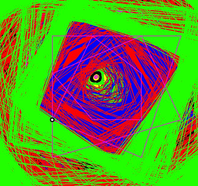
View/Sys/Gal: EMap "star out & star in, variation as EMap" in "OdeFactoryExs." This system of odes is defined by the equations: dx/dt = -.5*(x^2-y^2-1)+p, dy/dt = -x*y+q Parameters are: p = .93; q = .52; In this variation the iteration is of the classic Mandelbrot form: z <- z^2+c where z = x+i*y and c = p+i*q. The current values of p and q produce an interesting fractal called a Julia set. To zoom-in on any part of the fractal, position the cursor on a point of interest, then with the control key down, move the cursor to get a selection circle about the point. Release the control key and click the Update button in the Graphics Settings window. To cycle back to the ode view, click the Ode button. You can adjust parameters p and q to get various Julia sets. See the next version of the system.
|
|
View/Sys/Gal: EMap "star out & star in, variation as EMap, ver 2" in "OdeFactoryExs." This system of odes is defined by the equations: dx/dt = -.5*(x^2-y^2-1)+p, dy/dt = -x*y+q Parameters are: p = -.44; q = -1.40; Ver 3 shows another way to generate different fractals based on this system. Try some different color tables.
|
|
View/Sys/Gal: EMap "star out & star in, variation as EMapCT7, ver 3" in "OdeFactoryExs." This system of odes is defined by the equations: dx/dt = -.5*(x^2-y^2-b), dy/dt = -a*x*y Parameters are: a = 2.30; b = 1.10; This is another way to introduce control parameters into the original system. It produces fractals that differ from the classic fractals generated by the Mandelbrot iteration. Open the parameter controller and set a = 9.7 and b = -.4 then open the parameter controller again (to refine the b range to [-1,1]) and set b = -.37 then zoom in.
|
|
View/Sys/Gal: Ode "three limit cycles" in "OdeFactoryExs." This system of odes is defined by the equations: dx/dt = -y+cos(2*x)-.05*x, dy/dt = x+sin(2*y)-.05*y It looks like this system has exactly three limit cycles. To see the two ω-limit cycles, clear the view then click the "Flow" button. Start 50 random dots at max speed in +t and watch what happens. You can add 50 more dots while the animation runs by clicking more than once on the "Start Flow" button. To see the α-limit cycle, run the animation in -t. Another way to see the limit cycles is to go to the 3D/(x,y) view. The ω-limit cycles show up with red dots and the α-limit cycle shows up with blue dots. Can you prove there are exactly two three cycles? What if you replace the .05 in the equations with a parameter b = .05 then adjust b? Try the EMap view.
|
|
View/Sys/Gal: EMap "three limit cycles EMapCT5" in "OdeFactoryExs." This iteration is defined by: x <- -y+cos(2*x)-.05*x, y <- x+sin(2*y)-.05*y. EMap CT: 5
|
|
View/Sys/Gal: Ode "y' = -4*e^(-3*x)" in "OdeFactoryExs." This ode is defined by the equation: dx/dt = -4*e^(-3*t) in the (t,x) coordinate system. The 1st order 1D system corresponds to the 1st order ode y' = -4*e^(-3*x) in the (x,y) coordinate system. WA gives: x(t) = c_1+(4 e^(-3 t))/3 as the solution.
|
|
View/Sys/Gal: Ode "y' = -M/N, M=x+2; N=x^2" in "OdeFactoryExs." This ode is defined by the equation: dx/dt = -M/N in the (t,x) coordinate system. The 1st order 1D system corresponds to the 1st order ode y' = -M/N in the (x,y) coordinate system. Functions are: M=x+2; N=x^2 NOTE: User defined functions must always be defined in (t,x,y,z,w) coordinates.
|
|
View/Sys/Gal: Ode "y' = y*x-y^2-x" in "OdeFactoryExs." This ode is defined by the equation: dx/dt = x*t-x^2-t in the (t,x) coordinate system. The 1st order 1D system corresponds to the 1st order ode y' = y*x-y^2-x in the (x,y) coordinate system. Copy/paste this into WolframAlpha to see the closed form solution.
|
|
View/Sys/Gal: Ode "y'' = y+y'+a+P, a=5, P=x*y" in "OdeFactoryExs." This system of odes is defined by the equations: dx/dt = y, dy/dt = x+y+a+P in the (t,x,y) coordinate system. The 1st order 2D system corresponds to the 2nd order ode y'' = y+y'+a+P in the (x,y,y') coordinate system. Parameters are: a = 5 Functions are: P = x*y NOTE: User defined functions must always be defined in (t,x,y,z,w) coordinates.
| ||||||||||||||||||||||||||||