Click on an image to go directly to a system or scroll to see the systems in this gallery.
 |
 |
 |
 |
 |
 |
 |
 |
 |
 |
 |
 |
 |
 |
 |
 |
 |
 |
 |
 |
 |
 |
 |
 |
 |
 |
 |
 |
 |
 |
 |
 |
 |
 |
 |
 |
 |
 |
 |
 |
 |
 |
 |
 |
 |
 |
 |
 |
 |
 |
 |
 |
 |
 |
 |
 |
 |
 |
 |
 |
 |
 |
 |
 |
 |
 |
| OdeFactory Images and Annotations | ||||||||||||||||||||||||||||||||||||||||||||||||||||||||||||||||||||||||||||||||||||||||||||||||||||||||||||||||||||||||||||||||||||||||||||||||||||||||||||||||||||||||||||||
|
|
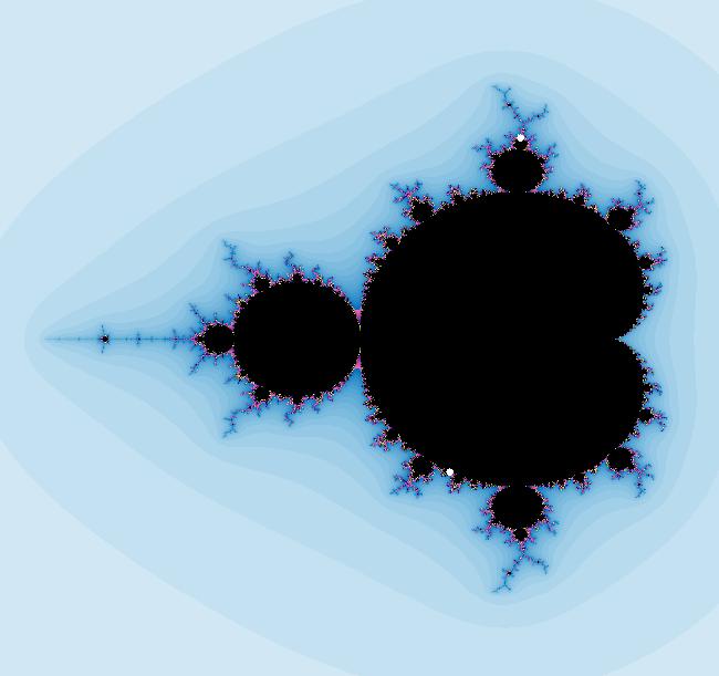
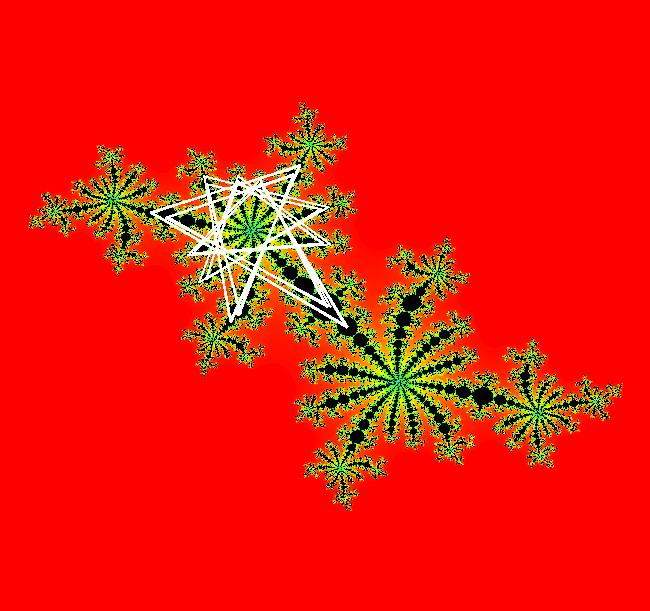
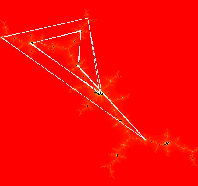
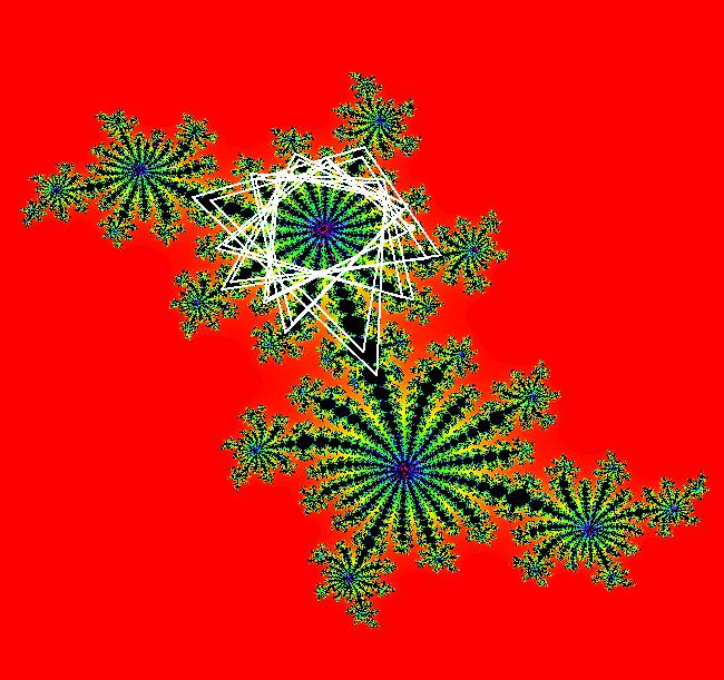
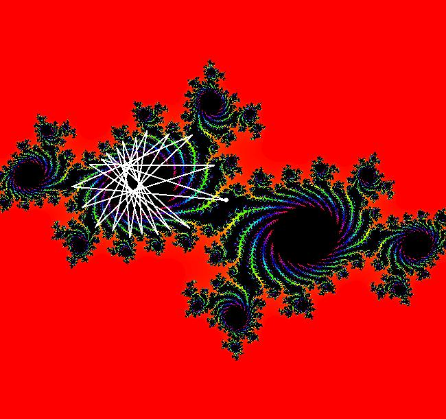
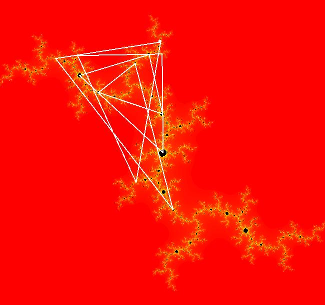
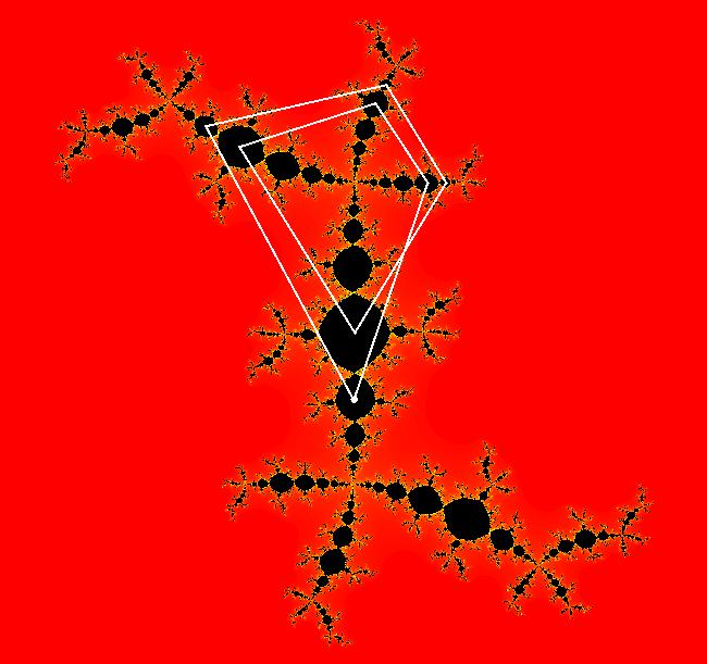
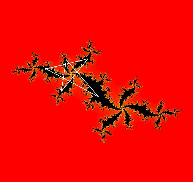
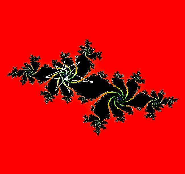
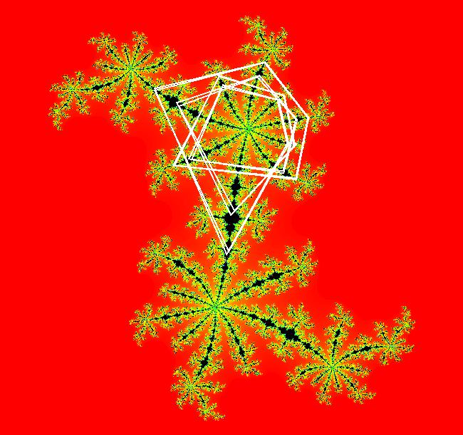
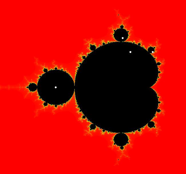
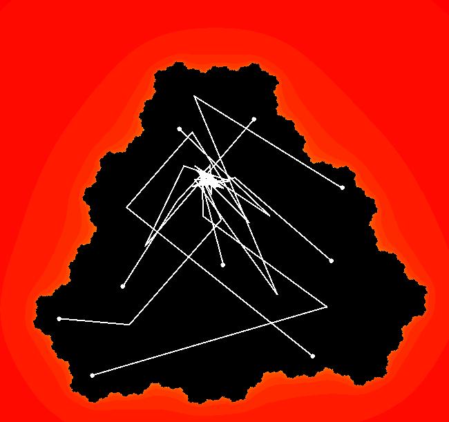
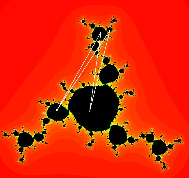
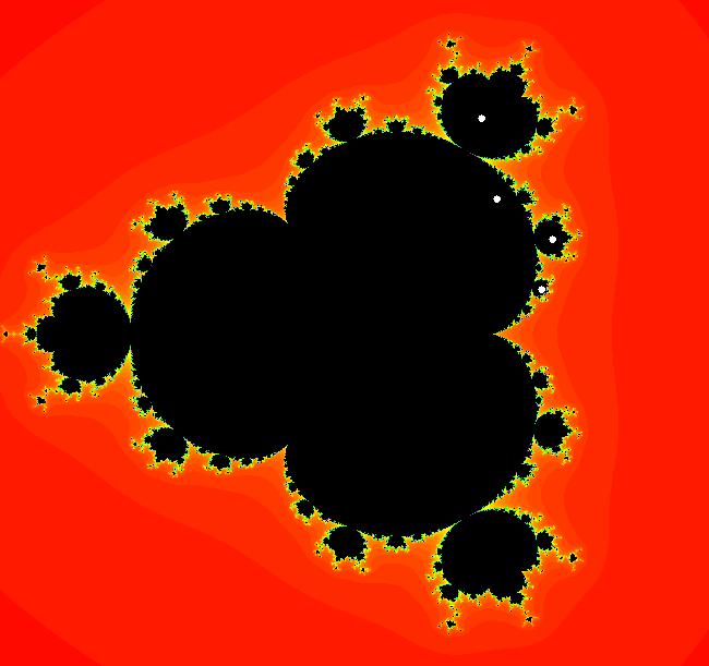
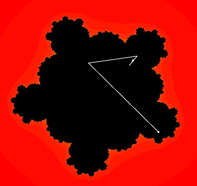
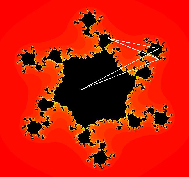
View/Sys/Gal: EMap " Mandelbrot: (x,y,z^2-w^2+x,2*z*w+y) EMapCT3" in "ClassicFractals." System 1 (complex, Julia set): z <- z^2+p+i*q using WA gives system 2 (real, 2D2P, Julia set) : x <- x^2-y^2+p, y <- 2*x*y+q using 4D0P gives system 3 ((x,y) EMap view, Mandelbrot set): x <- x, x is "p" y <- y, y is "q" z <- z^2-w^2+x, w <- 2*z*w+y. There have been many books and technical articles written about the Mandelbrot set and the associated Julia sets. For a nice introduction to the Mandelbrot set see Wikipedia. From the "Chaos and Fractals" book by Peitgen/Jurgens/Saupe p. 867: "The buds of the Mandelbrot set correspond to the Julia sets that bound basins of attraction of periodic orbits." Most often there is a single periodic attractor in a Julia set however for the Siegel disk system there is an infinite number of periodic orbits. The larger the bud on the Mandelbrot set the smaller the period of the corresponding Julia set. If we number the primary buds (the ones on the main cardioid) in decreasing size, starting with 2 for the west bud and work clockwise, the bud number (bud#) will be the period of the corresponding Julia set. Using the same procedure with secondary buds the Julia set periods will be the products of the primary and secondary bud numbers. Each primary bud ends with an n-petal antennae. For any n, there many different Julia sets of period n. There are Julia sets of all periods. A bud#, or bud address, in the following table is the primary bud number multiplied by secondary bud numbers. For example, bud# 3*2*2 means go to bud# 3, then go to bud# 3's bud# 2 then go to bud# 2's bud# 2.
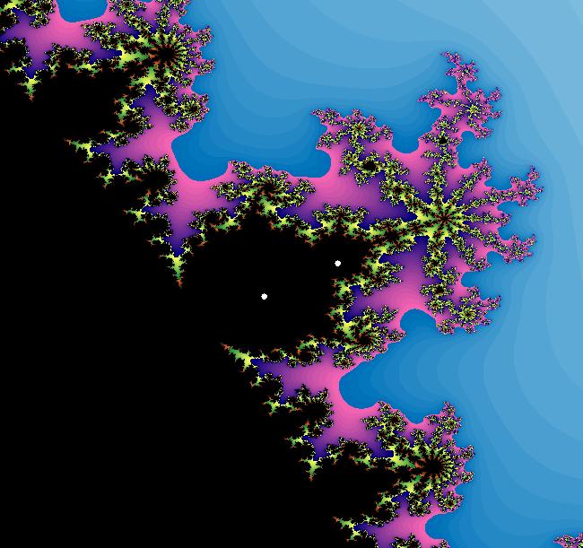
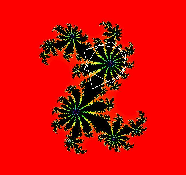
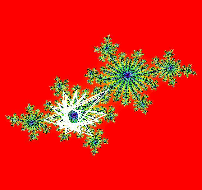
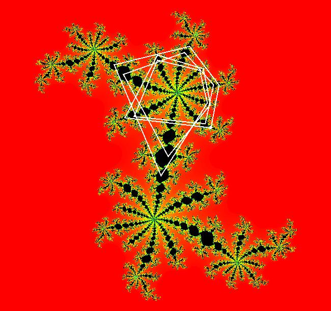
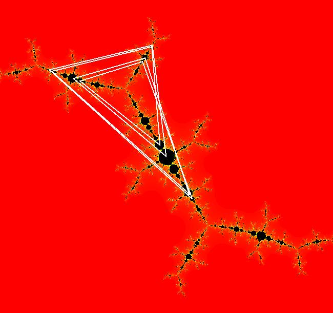
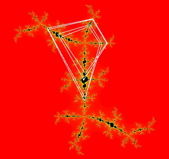
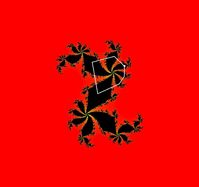
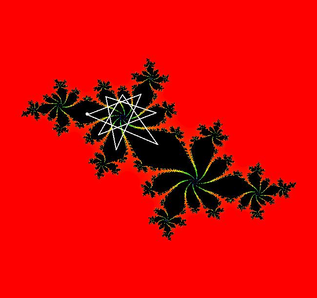
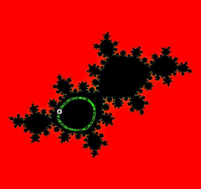
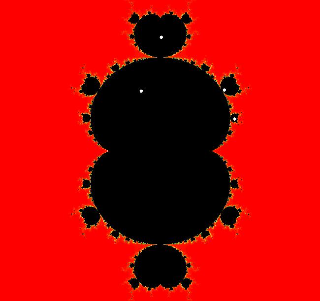
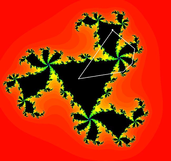
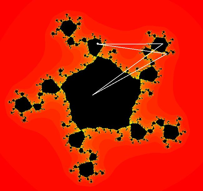
The last entry, S, stands for the Siegel disk system. Image 1: The white dots in the (x,y) view show the locations of bud# 3*2*2 and bud# S. Image 2: The white dots in the zoomed in (x,y) view show the locations of bud# 9 and bud# 9*2.
|
|
View/Sys/Gal: EMap "Julia 1 EMapMax" in "ClassicFractals." This iteration is defined by: x <- x^2-y^2+p, y <- 2*x*y+q. Parameters are: p = .0000; q = .5000; EMap CT: 0 This is a Julia set for bud# 1. Image 1: Fixed point attractor at (-0.136010,0.393076).
|
|
View/Sys/Gal: EMap "Julia 11 EMapMax" in "ClassicFractals." This iteration is defined by: x <- x^2-y^2+p, y <- 2*x*y+q. Parameters are: p = -.301; q = .63; EMap CT: 0 Image 1: An 11-petal fractal with a per-11 attractor.
|
|
View/Sys/Gal: EMap "Julia 11*2 EMapMax" in "ClassicFractals." This iteration is defined by: x <- x^2-y^2+p, y <- 2*x*y+q. Parameters are: p = -.296; q = .643; EMap CT: 0 Image 1: An 11-petal 2-petal fractal with a per-11*2=22 attractor.
|
|
View/Sys/Gal: EMap "Julia 13 EMapMax" in "ClassicFractals." This iteration is defined by: x <- x^2-y^2+p, y <- 2*x*y+q. Parameters are: p=.37632; q=.17704 EMap CT: 0 Image 1: A 13-petal fractal with a per-13 attractor.
|
|
View/Sys/Gal: EMap "Julia 13b EMapMax" in "ClassicFractals." This iteration is defined by: x <- x^2-y^2+p, y <- 2*x*y+q. Parameters are: p = -.714; q = .238; EMap CT: 0 Image 1: Another 13-petal fractal with a per-13 attractor.
|
|
View/Sys/Gal: EMap "Julia 13*2 EMapMax" in "ClassicFractals." This iteration is defined by: x <- x^2-y^2+p, y <- 2*x*y+q. Parameters are: p=.379796; q=.1762036 EMap CT: 0 Image 1: A 13-petal 2-petal fractal with a per-13*2 = 26 attractor.
|
|
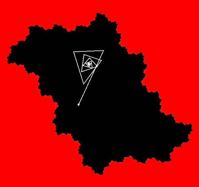
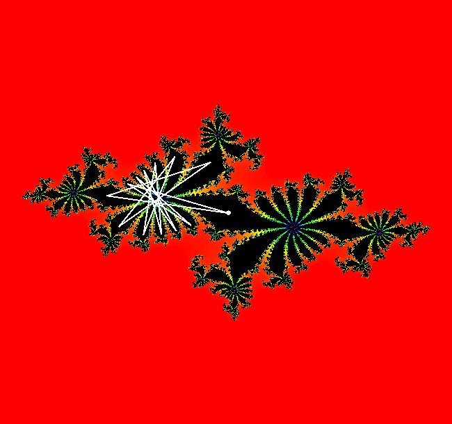
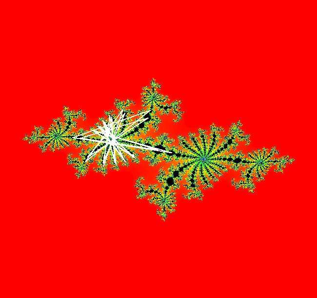
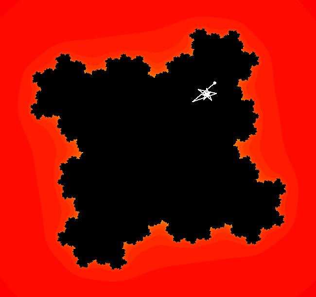
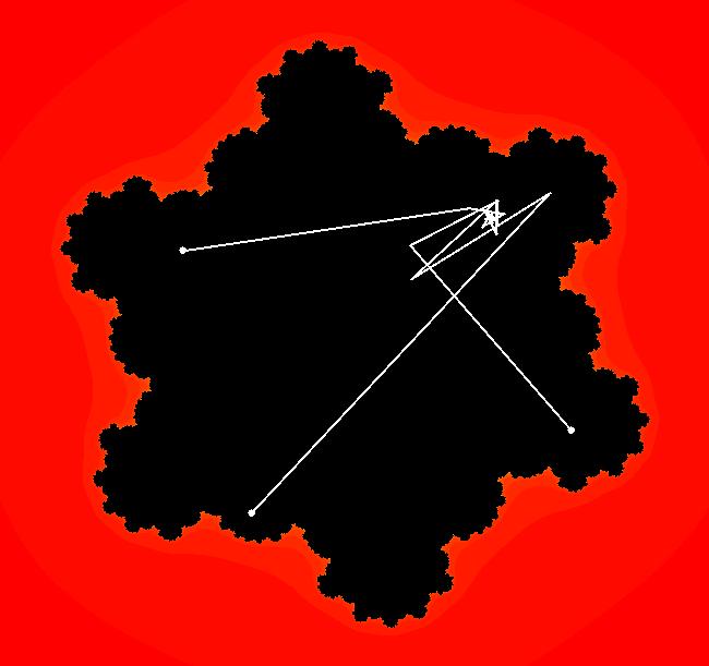
View/Sys/Gal: EMap "Julia 14 EMapMax" in "ClassicFractals." This iteration is defined by: x <- x^2-y^2+p, y <- 2*x*y+q. Parameters are: p = -.129; q = .988; EMap CT: 0 (p,q) = (-.129,.988) is in the disconnected antennae of bud# 3 of the Mandelbrot set on the left side. The Julia set is fractal and not connected. Image 1: There is a per-14 attractor with a point at (-0.230280,0.358334) which is near the center of the largest fragment of the Julia set. The next two largest parts of the Julia set are at the fixed points of the system in the Ode view.
|
|
View/Sys/Gal: EMap "Julia 18*2*2 EMapMax" in "ClassicFractals." This iteration is defined by: x <- x^2-y^2+p, y <- 2*x*y+q. Parameters are: p=-.4311309; q=-.574954 EMap CT: 0 Image 1: An 18-petal and two 2-petal fractal with a per-18*2*2=72 attractor.
|
|
View/Sys/Gal: EMap "Julia 2 EMapMax" in "ClassicFractals." This iteration is defined by: x <- x^2-y^2+p, y <- 2*x*y+q. Parameters are: p=-1; q=0 EMap CT: 0 Image 1: A 2-petal fractal with a per-2 attractor.
|
|
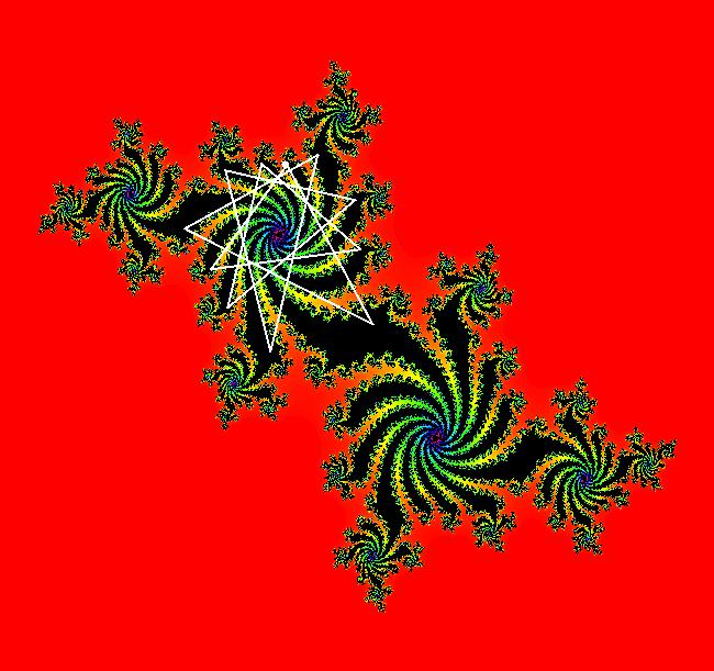
View/Sys/Gal: EMap "Julia 2*13 EMapMax" in "ClassicFractals." This iteration is defined by: x <- x^2-y^2+p, y <- 2*x*y+q. Parameters are: p = -.721; q = .239; EMap CT: 0 per-2*13=26 orbit at (-0.279378,-0.080727) Image 1: A 2-petal 13-petal fractal with a per-2*13=26 attractor.
|
|
View/Sys/Gal: EMap "Julia 2*17 EMapMax" in "ClassicFractals." This iteration is defined by: x <- x^2-y^2+p, y <- 2*x*y+q. Parameters are: p = .078; q = .619; EMap CT: 0 Image 1: A 2-petal 17-petal fractal with a per-2*17=34 attractor.
|
|
View/Sys/Gal: EMap "Julia 2*2 EMapMax" in "ClassicFractals." This iteration is defined by: x <- x^2-y^2+p, y <- 2*x*y+q. Parameters are: p=-1.31; q=0 EMap CT: 0 Image 1: Two 2-petal fractals with a per-2*2=4 attractor.
|
|
View/Sys/Gal: EMap "Julia 2*3 EMapMax" in "ClassicFractals." This iteration is defined by: x <- x^2-y^2+p, y <- 2*x*y+q. Parameters are: p=-1.1313; q= .2232 EMap CT: 0 Image 1: A 2-petal 3-petal fractal with a per-2*3=6 attractor.
|
|
View/Sys/Gal: EMap "Julia 2*9 EMapMax" in "ClassicFractals." This iteration is defined by: x <- x^2-y^2+p, y <- 2*x*y+q. Parameters are: p = .339; q = .415; EMap CT: 0 Image 1: A 2-petal 9-petal fractal with a per-2*9=18 attractor.
|
|
View/Sys/Gal: EMap "Julia 20 EMapMax" in "ClassicFractals." This iteration is defined by: x <- x^2-y^2+p, y <- 2*x*y+q. Parameters are: p = -.6800; q = .3000; EMap CT: 0 Image 1: A 20-petal fractal with a per-20 attractor.
|
|
View/Sys/Gal: EMap "Julia 3 EMapMax" in "ClassicFractals." This iteration is defined by: x <- x^2-y^2+p, y <- 2*x*y+q. Parameters are: p=-.1; q=.7 EMap CT: 0 Image 1: A 3-petal fractal with a per-3 attractor.
|
|
View/Sys/Gal: EMap "Julia 3*2 EMapMax" in "ClassicFractals." This iteration is defined by: x <- x^2-y^2+p, y <- 2*x*y+q. Parameters are: p=-.11271; q=.8457 EMap CT: 0 Image 1: A 3-petal 2-petal fractal with a per-3*2=6 attractor.
|
|
View/Sys/Gal: EMap "Julia 3*2*2 EMapMax" in "ClassicFractals." This iteration is defined by: x <- x^2-y^2+p, y <- 2*x*y+q. Parameters are: p=-.1099; q=.88618 EMap CT: 0 Image 1: A 3-petal and two 2-petal fractals with a per = 3*2*2 = 12 attractor.
|
|
View/Sys/Gal: EMap "Julia 3*4 EMapMax" in "ClassicFractals." This iteration is defined by: x <- x^2-y^2+p, y <- 2*x*y+q. Parameters are: p = -.007; q = .806; EMap CT: 0 Image 1: A 3-petal 4-petal fractal with a per-3*4=12 attractor.
|
|
View/Sys/Gal: EMap "Julia 3*4b EMapMax" in "ClassicFractals." This iteration is defined by: x <- x^2-y^2+p, y <- 2*x*y+q. Parameters are: p = -.11; q = .886; EMap CT: 0 Image 1: Another 3-petal 4-petal fractal with a per-3*4=12 attractor.
|
|
View/Sys/Gal: EMap "Julia 3b EMapMax" in "ClassicFractals." This iteration is defined by: x <- x^2-y^2+p, y <- 2*x*y+q. Parameters are: p = -.1800; q = .8000; EMap CT: 0 Image 1: Another 3-petal fractal with a per-3 attractor.
|
|
View/Sys/Gal: EMap "Julia 4 EMapMax" in "ClassicFractals." This iteration is defined by: x <- x^2-y^2+p, y <- 2*x*y+q. Parameters are: p=.3; q=.5 EMap CT: 0 Image 1: A 4-petal fractal with a per-4 attractor.
|
|
View/Sys/Gal: EMap "Julia 4*2 EMapMax" in "ClassicFractals." This iteration is defined by: x <- x^2-y^2+p, y <- 2*x*y+q. Parameters are: p = .325; q = .563; EMap CT: 0 Image 1: A 4-petal 2-petal fractal with a per-4*2=8 attractor.
|
|
View/Sys/Gal: EMap "Julia 4*2*2 EMapMax" in "ClassicFractals." This iteration is defined by: x <- x^2-y^2+p, y <- 2*x*y+q. Parameters are: p = .336; q = .57; EMap CT: 0 Image 1: A 4-petal 2-petal 2-petal fractal with a per-4*2*2=16 attractor.
|
|
View/Sys/Gal: EMap "Julia 4b EMapMax" in "ClassicFractals." This iteration is defined by: x <- x^2-y^2+p, y <- 2*x*y+q. Parameters are: p = .2400; q = .5300; EMap CT: 0 Image 1: Another 4-petal fractal with a per-4 attractor.
|
|
View/Sys/Gal: EMap "Julia 5 EMapMax" in "ClassicFractals." This iteration is defined by: x <- x^2-y^2+p, y <- 2*x*y+q. Parameters are: p=.379; q=.329 EMap CT: 0 Image 1: A 5-petal fractal with a per-5 attractor.
|
|
View/Sys/Gal: EMap "Julia 5b EMapMax" in "ClassicFractals." This iteration is defined by: x <- x^2-y^2+p, y <- 2*x*y+q. Parameters are: p = -.5000; q = .6000; EMap CT: 0 Image 1: Another 5-petal fractal with a per-5 attractor.
|
|
View/Sys/Gal: EMap "Julia 6 EMapMax" in "ClassicFractals." This iteration is defined by: x <- x^2-y^2+p, y <- 2*x*y+q. Parameters are: p=.39; q=.211 EMap CT: 0 Image 1: A 6-petal fractal with a per-6 attractor.
|
|
View/Sys/Gal: EMap "Julia 6b EMapMax" in "ClassicFractals." This iteration is defined by: x <- x^2-y^2+p, y <- 2*x*y+q. Parameters are: p = .4000; q = .2100; EMap CT: 0 Image 1: Another 6-petal fractal with a per-6 attractor.
|
|
View/Sys/Gal: EMap "Julia 7 EMapMax" in "ClassicFractals." This iteration is defined by: x <- x^2-y^2+p, y <- 2*x*y+q. Parameters are: p=.3726; q=.1378 EMap CT: 0 Image 1: A 7-petal fractal with a per-7 attractor.
|
|
View/Sys/Gal: EMap "Julia 7b EMapMax" in "ClassicFractals." This iteration is defined by: x <- x^2-y^2+p, y <- 2*x*y+q. Parameters are: p = -.6200; q = .4100; EMap CT: 0 Image 1: Another 7-petal fractal with a per-7 attractor.
|
|
View/Sys/Gal: EMap "Julia 8 EMapMax" in "ClassicFractals." This iteration is defined by: x <- x^2-y^2+p, y <- 2*x*y+q. Parameters are: p = -.3600; q = .6100; EMap CT: 0 Image 1: An 8-petal fractal with a per-8 attractor.
|
|
View/Sys/Gal: EMap "Julia 9 EMapMax" in "ClassicFractals." This iteration is defined by: x <- x^2-y^2+p, y <- 2*x*y+q. Parameters are: p = .3300; q = .4100; EMap CT: 0 Image 1: A 9-petal fractal with a per-9 attractor.
|
|
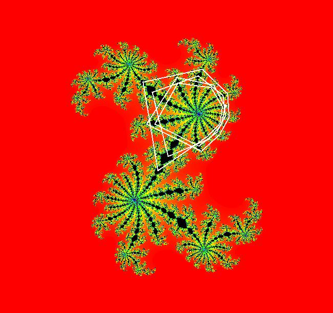
View/Sys/Gal: EMap "Julia 9*2 EMapMax" in "ClassicFractals." This iteration is defined by: x <- x^2-y^2+p, y <- 2*x*y+q. Parameters are: p = .339; q = .4151; EMap CT: 0 Image 1: A 9-petal 2-petal fractal with a per-9*2=18 attractor.
|
|
View/Sys/Gal: EMap "Julia 9*2*2 EMapMax" in "ClassicFractals." This iteration is defined by: x <- x^2-y^2+p, y <- 2*x*y+q. Parameters are: p = .341; q = .417; EMap CT: 0 Image 1: A 9-petal 2-petal 2-petal fractal with a per-9*2*2=36 attractor.
|
|
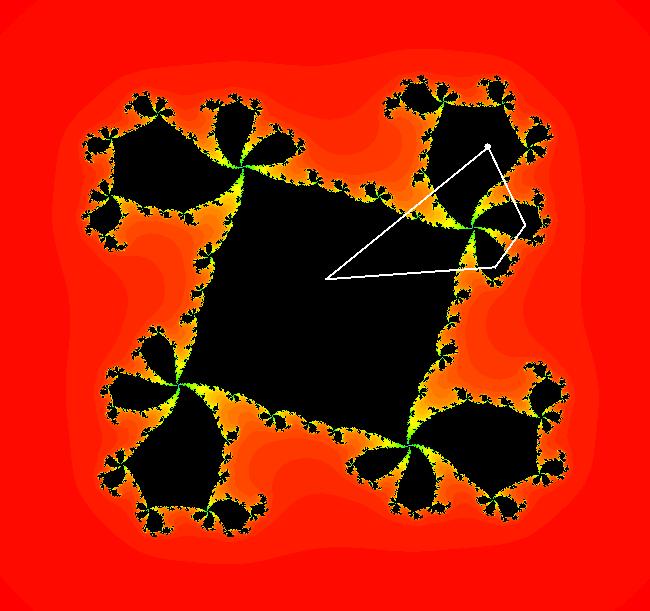
View/Sys/Gal: EMap "Julia S EMapMax" in "ClassicFractals." This iteration is defined by: x <- x^2-y^2+p, y <- 2*x*y+q. Parameters are: p = -.3905407802; q = -.58678790073; EMap CT: 0 This is the Siegal disk example. All orbits are attracted to rings about the point: (-0.368684,-0.337745) in the lower-left large region. The rings are periodic orbits with large periods. For example, the ring at (-0.368696,-0.337804), which looks like a point unless you zoom way in, has period 55. Image 1: Running a Flow shows a sample ring.
|
|
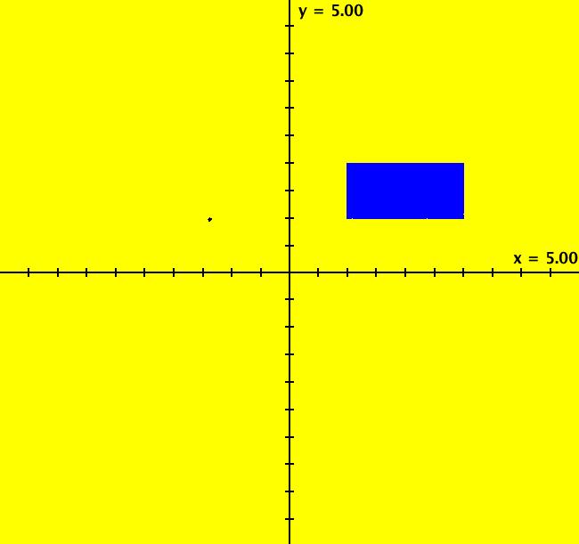
View/Sys/Gal: IMap "R (random(1,3),random(1,2)) IMap0100" in "ClassicFractals." The four "R" systems are tests of the OdeFactory random(a,b) function. The OdeFactory random function is defined as: random(a,b) = (b-a)*Math.random()+a where Math.random() is the Java random function which generates a random number in the interval [0,1). On a pixelated computer screen, [0,1) is the same as (0,1) or [0,1] so random(0,1) is Math.random(). The iteration is defined by: x <- random(1,3), y <- random(1,2). Image 1: Since x is in (1,3) and y is in (1,2), we get a 2 by 1 rectangle, with a corner at (1,1), in the IMap view.
|
|
View/Sys/Gal: IMap "R (round(random(.5,3.5)-2),2*(1-abs(x))) IMap1000" in "ClassicFractals." This iteration is defined by: x <- round(random(.5,3.5)-2), y <- 2*(1-abs(x)). random(.5,3.5)-2 is in (-1.5,1.5) so round(random(.5,3.5)-2) is -1, 0 or 1 with equal probability. You might expect to get just the three points (-1,0), (0,2) and (1,0) but we actually get six points (-1,0) and (-1,2) if prev x was 0, (0,2) and (0,0) if prev x was +-1, (1,0) and (1,2) if prev x was 0. Recall that the system is "atomic," so when computing the new left hand sides the previous right hand sides are used. The "<-" notation is just shorthand for: x(n+1) = round(random(.5,3.5)-2), y(n+1) = 2*(1-abs(x(n))). So if x(n+1) = -1, y(n+1) will be 2 and we get (-1,2). Image 1: The 6 points: (-1,0), (0,0), (1,0), (-1,2), (0,2) and (1,2).
|
|
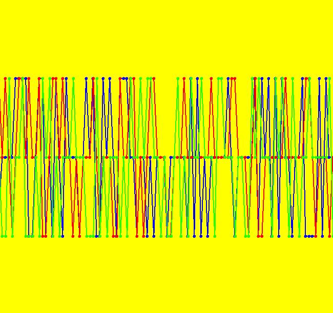
View/Sys/Gal: IMap "R (round(random(1,3))) IMap" in "ClassicFractals." This iteration is defined by: x <- round(random(1,3)). After the first hop, x is 1, 2 or 3 but probability(3) = .25, probability(2) = .5 and probability(1) = .25 since the round function rounds to the nearest integer. Image 1: This is a plot of (t,x) points from t = 1 to 100. The bottom and top rows of dots are at x = 1 and x = 3 and the denser middle row is at x = 2.
|
|
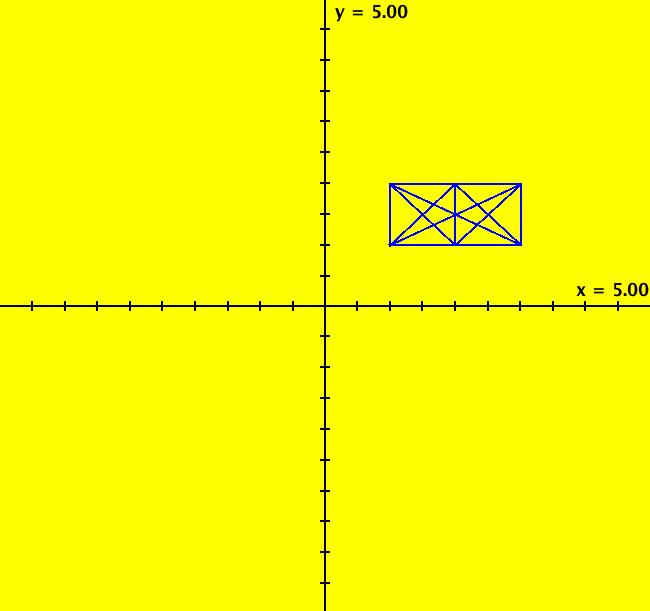
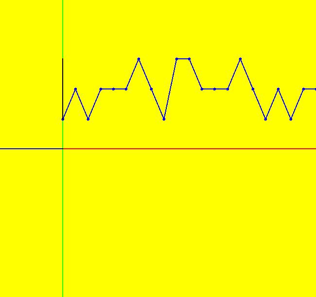
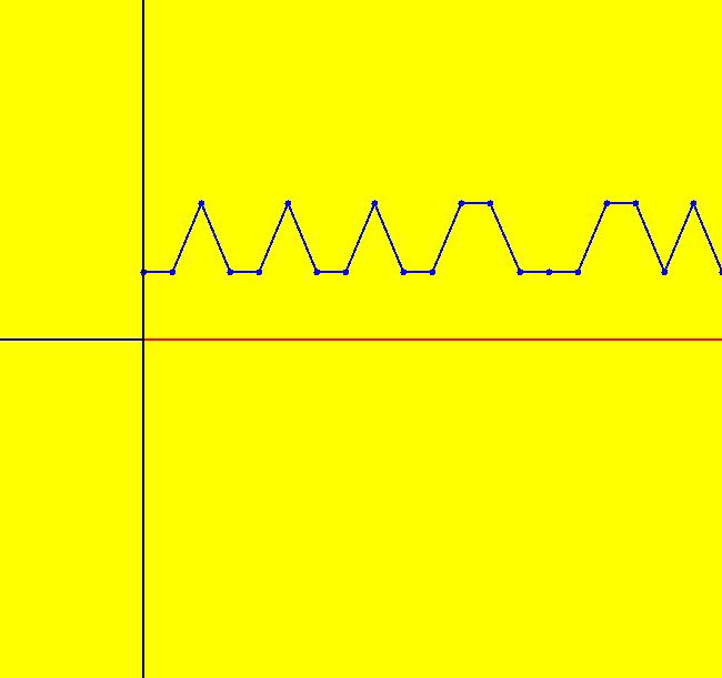
View/Sys/Gal: IMap "R (round(random(1,3)),round(random(1,2))) IMap1000" in "ClassicFractals." This iteration is defined by: x <- round(random(1,3)), y <- round(random(1,2)). (x,y) is: (1,1), (1,2), (2,1), (2,2), (3,1), (3,2). The six (x,y) points are the attractor set. Image 1: The IMap1000 image shows the connections between the six points. Image 2: The 3D/(t,x) view. Image 3: The 3D/(t,y) view.
|
|
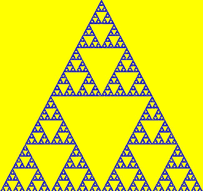
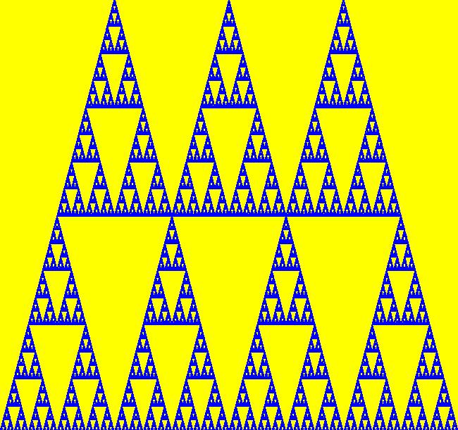
View/Sys/Gal: IMap "Sierpinski gasket, IMap0010" in "ClassicFractals." This system is defined by: x <- (x+z)/2, y <- (y+w)/2, z <- round(random(.5,3.5)-2), w <- 2*(1-abs(z)). In this example the algorithm is probabilistic. The chaotic orbit is not deterministic but the resulting image is a highly organized fractal. This is the (x,y) view and the ICs are: (x,y,z,w) = (0,0,-1,0). Image 1: For x in [-.25,.25] and y in [1,2], we have the Sierpinski gasket. For (z,w) we get (-1,0) and (-1,2) if prev z was 0, (0,2) and (0,0) if prev z was +-1, (1,0) and (1,2) if prev z was 0. The (x,y) iterates are in the 2 by 2 square centered at (x,y) = (0,1). Zoom out to see the full image. Image 2: The full image in the 2 by 2 square: -1 <= x <= 1, 0 <= y <= 2. For a discussion of the generating algorithm, see section 6.1 of the Peitgen/Jurgens/Saupe book. PJS call this a "FRCM" (Fortune Wheel Reduction Copy Machine). Here it is implemented by what PJS might call a "FIFS" (Fortune Wheel Iterated Function System).
|
|
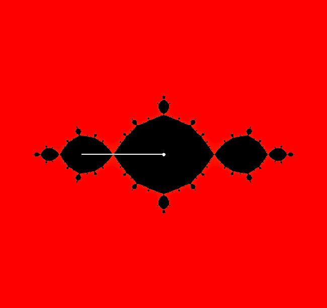
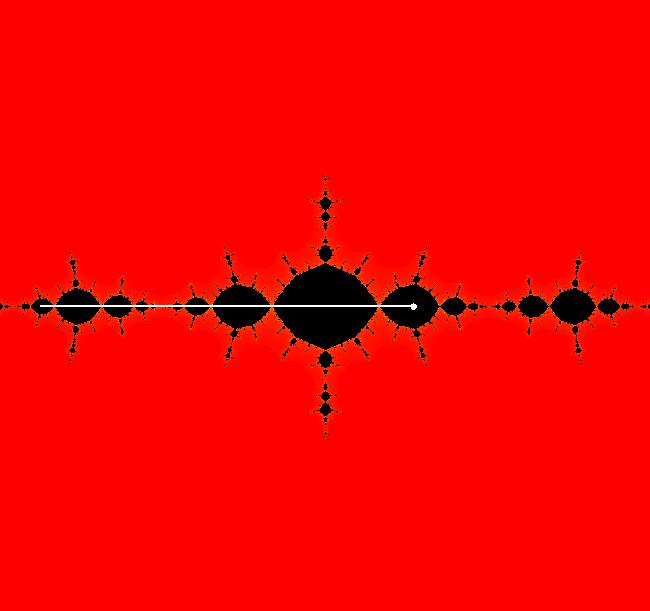
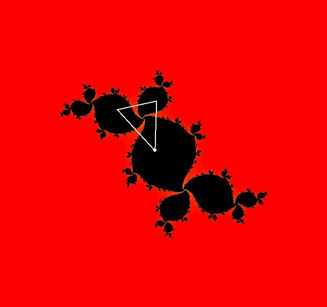
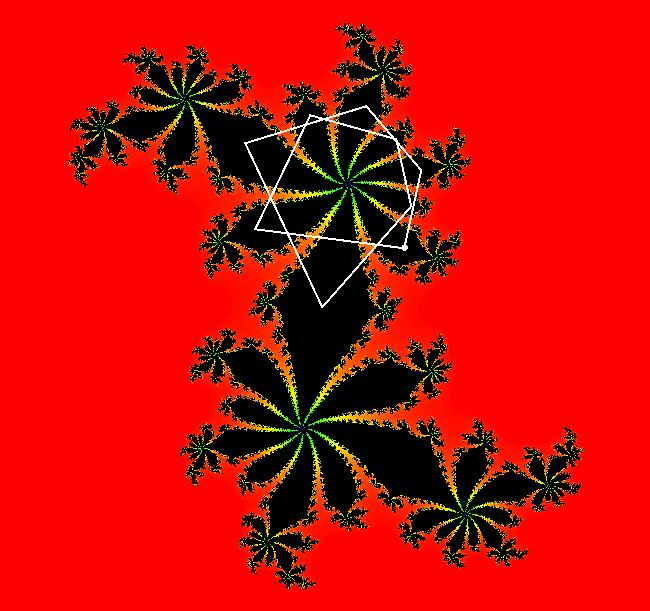
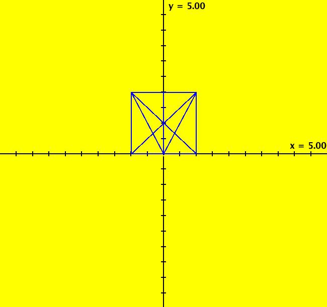
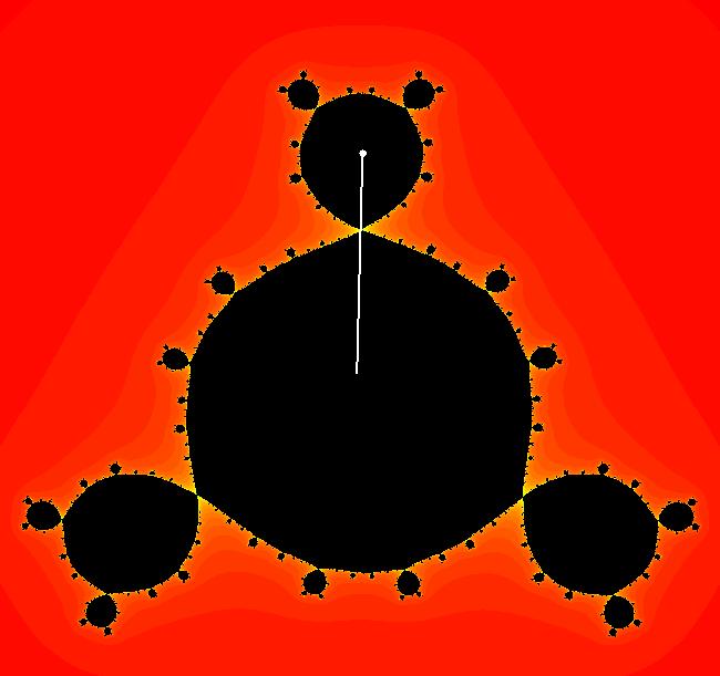
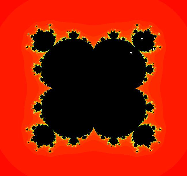
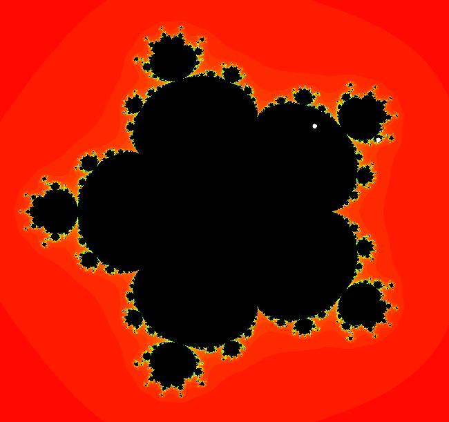
View/Sys/Gal: EMap "z^2+c, bifurcation diagram, EMapMax" in "ClassicFractals." The bifurcation diagram for the complex iteration system: z <- z^2+c, c = p+i*q, generated by the corresponding 4D real system in the (x,y) = "(p,q)" plane, x <- x, y <- y, z <- z^2-w^2+x, w <- 2*z*w+y. is the filled Mandelbrot set. Image 1: (p,q) values in the filled Mandelbrot corresponding to Julia sets with attractors with: per-1, (p,q) = (0,.5), per-2, (p,q) = (-1,0), per-3, (p,q) = (-.1,.7), per-4, (p,q) = (.3,.5). The bud numbering algorithm: bud 1 <-> large main region, bud 2 <-> largest bud at π/1, bud 3 <-> next largest bud, cw, bud 4 <-> next largest bud, cw... gives the period of the attractor for the Julia set with (p,q) in the corresponding bud. Image 1: Mandelbrot set with (p,q) in buds: 1, 2, 3, 4. The question is - does the bud numbering algorithm give the period of the attractor for the Julia set with (p,q) in the corresponding bud for:
z <- z^n+c, with c = p+i*q, when n is an integer > 2? The following examples seem to suggest that it does.
|
|
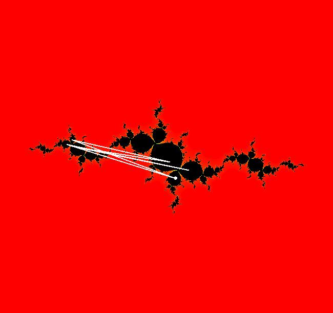
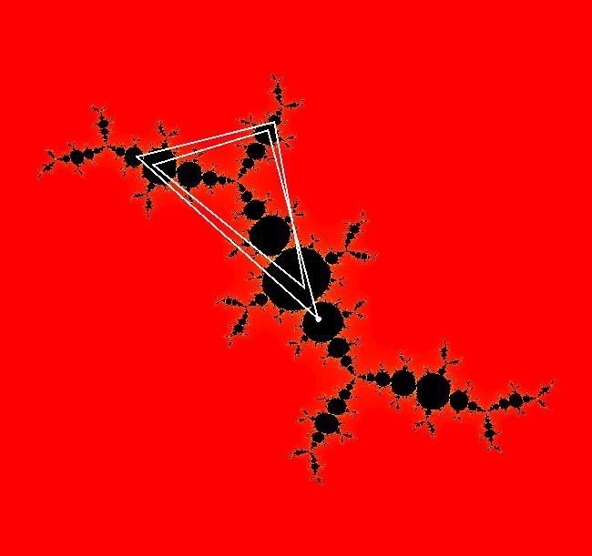
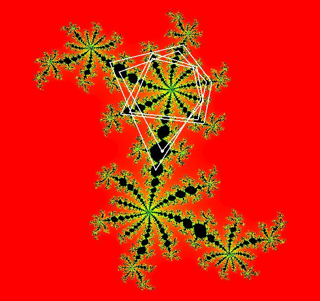
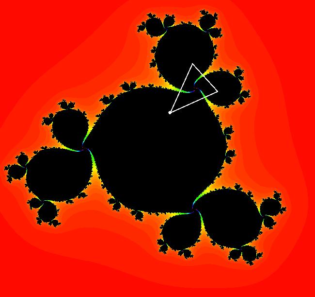
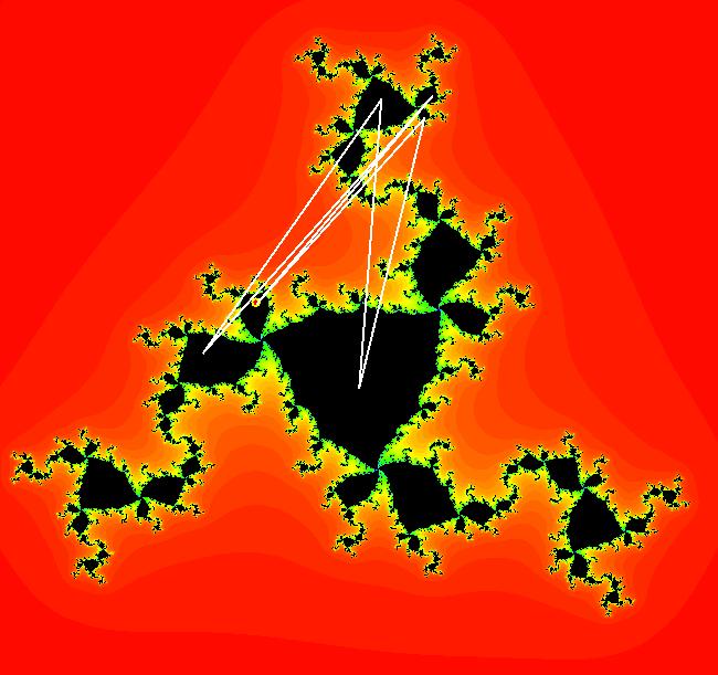
View/Sys/Gal: EMap "z^3+c, bifurcation diagram, EMapMax" in "ClassicFractals." This system is defined by: x <- x, y <- y, z <- z*(z^2-3*w^2)+x, w <- w*(3*z^2-w^2)+y. Bifurcation diagram for: z <- z^3+c The buds are similar to the buds on the Mandelbrot set and can be numbered (addressed) in the same way: bud 1 is the main region bud 2 is at π/2, bud 3 is the next largest bud cw, bud 4 is the next largest bud cw ... Image 1: z^3+c bifurcation diagram showing: per-1 <-> (p,q) = (-.145706,.490276), per-2 <-> (p,q) = (.007669,.931929), per-3 <-> (p,q) = (.5,.5), per-4) <-> (p,q) = (.578988,.263371).
|
|
View/Sys/Gal: EMap "z^3+c, per-1, p=-0.145706; q=0.490276, EMap" in "ClassicFractals." This iteration is defined by: x <- x*(x^2-3*y^2)+p, y <- y*(3*x^2-y^2)+q. Parameters are: p=-0.145706; q=0.490276 EMap CT: 0 Image 1: per-1 attractor at: (x,y) = (-0.095053,0.425020).
|
|
View/Sys/Gal: EMap "z^3+c, per-2, p=0.007669; q=0.931929, EMap" in "ClassicFractals." This iteration is defined by: x <- x*(x^2-3*y^2)+p, y <- y*(3*x^2-y^2)+q. Parameters are: p=0.007669; q=0.931929 EMap CT: 0 Image 1: per-2 attractor at: (x,y) = (0.008355,0.929907).
|
|
View/Sys/Gal: EMap "z^3+c, per-3, p=.5; q=.5, EMap" in "ClassicFractals." This iteration is defined by: x <- x*(x^2-3*y^2)+p, y <- y*(3*x^2-y^2)+q. Parameters are: p=.5; q=.5 EMap CT: 0 Image 1: per-3 attractor at: (x,y) = (0.099053,0.302113).
|
|
View/Sys/Gal: EMap "z^3+c, per-4, p=0.578988; q=0.263371, EMap" in "ClassicFractals." This iteration is defined by: x <- x*(x^2-3*y^2)+p, y <- y*(3*x^2-y^2)+q. Parameters are: p=0.578988; q=0.263371 EMap CT: 0 Image 1: per-4 attractor at: (x,y) = (0.347874,0.783155).
|
|
View/Sys/Gal: EMap "z^3+c, per-4=2*2. p=0.203221; q=1.077796, EMap" in "ClassicFractals." This iteration is defined by: x <- x*(x^2-3*y^2)+p, y <- y*(3*x^2-y^2)+q. Parameters are: p=0.203221; q=1.077796 EMap CT: 0 Image 1: per-4=1*2*2 attractor at: (x,y) = (-0.496912,-0.038076).
|
|
View/Sys/Gal: EMap "z^3+c, per-5, p=0.548313; q=0.141815, EMap" in "ClassicFractals." This iteration is defined by: x <- x*(x^2-3*y^2)+p, y <- y*(3*x^2-y^2)+q. Parameters are: p=0.548313; q=0.141815 EMap CT: 0 Image 1: per-5 attractor at: (x,y) = (0.394341,0.778608).
|
|
View/Sys/Gal: EMap "z^3+c, per-6=2*3, p=0.226227; q=0.935981, EMap" in "ClassicFractals." This iteration is defined by: x <- x*(x^2-3*y^2)+p, y <- y*(3*x^2-y^2)+q. Parameters are: p=0.226227; q=0.935981 EMap CT: 0 Image 1: per-6=1*2*3 attractor at; (x,y) = (-0.357057,0.259281).
|
|
View/Sys/Gal: EMap "z^3+c, per-7, p=0.532672; q=0.094250, EMapMax" in "ClassicFractals." This iteration is defined by: x <- x*(x^2-3*y^2)+p, y <- y*(3*x^2-y^2)+q. Parameters are: p=0.532672; q=0.094250 EMap CT: 0 Image 1: per-7 attractor at: (x,y) = (0.772299,0.322592).
|
|
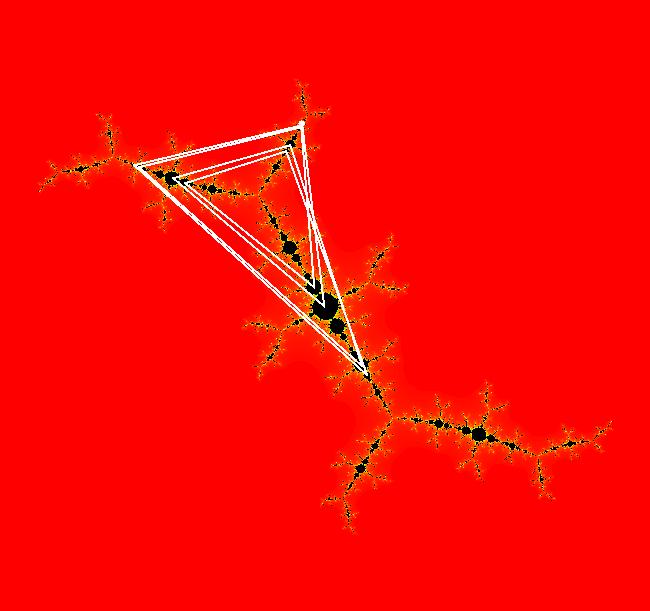
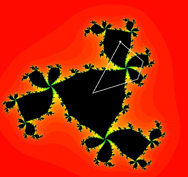
View/Sys/Gal: EMap "z^4+c, bifurcation diagram, EMap" in "ClassicFractals." This system is defined by: x <- x, y <- y, z <- z^4-6*z^2*w^2+w^4+x, w <- 4*z^3*w-4*z*w^3+y. Again, the buds are similar to the buds on the Mandelbrot set and can be numbered (addressed) in the same way: bud 1 is the main region bud 2 is at π/3, bud 3 is the next largest bud cw, bud 4 is the next largest bud cw ... Image 1: z^4+c bifurcation diagram showing: per-1 <-> (p,q) = (.5,.5), per-2 <-> (p,q) = (0.444785,0.802269), per-3 <-> (p,q) = (0.694018,0.352512), per-4 <-> (p,q) = (.6561845,.162075).
|
|
View/Sys/Gal: EMap "z^4+c, per-1, p=.5; q=.5, EMap" in "ClassicFractals." This iteration is defined by: x <- x^4-6*x^2*y^2+y^4+p, y <- 4*x^3*y-4*x*y^3+q. Parameters are: p=.5; q=.5 EMap CT: 0 Image 1: per-1 attractor at: (x,y) = (0.382154,0.456495).
|
|
View/Sys/Gal: EMap "z^4+c, per-4, p=0.651840; q=0.162075, EMap" in "ClassicFractals." This iteration is defined by: x <- x^4-6*x^2*y^2+y^4+p, y <- 4*x^3*y-4*x*y^3+q. Parameters are: p=0.651840; q=0.162075 EMap CT: 0 Image 1: per-4 attractor at: (x,y) = (0.623386,0.646358).
|
|
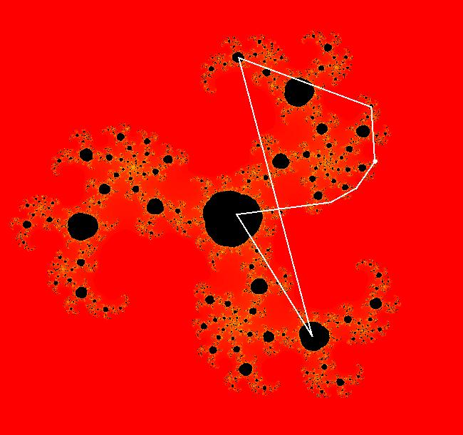
View/Sys/Gal: EMap "z^5+c, bifurcation diagram, EMap" in "ClassicFractals." This system is defined by: x <- x, y <- y, z <- z^5-10*z^3*w^2+5*z*w^4+x, w <- 5*z^4*w-10*z^2*w^3+w^5+y. Again, the buds are similar to the buds on the Mandelbrot set and can be numbered (addressed) in the same way: bud 1 is the main region bud 2 is at π/4, bud 3 is the next largest bud cw, bud 4 is the next largest bud cw ... Image 1: z^5+c bifurcation diagram showing: per-1 <-> (p,q) = (.5,.5), per-2 <-> (p,q) = (0.644172,0.700972), per-4=2*2 <-> (p,q) = (.801180,.547002).
|
|
View/Sys/Gal: EMap "z^5+c, per-1, p=.5; q=.5, EMap" in "ClassicFractals." This iteration is defined by: x <- x^5-10*x^3*y^2+5*x*y^4+p, y <- 5*x^4*y-10*x^2*y^3+y^5+q. Parameters are: p=.5; q=.5 EMap CT: 0 Image 1: per-1 attractor at: (x,y) = (0.436567,0.436567).
|
|
View/Sys/Gal: EMap "z^5+c, per-4=2*2, p=0.801380; q=0.547002, EMap" in "ClassicFractals." This iteration is defined by: x <- x^5-10*x^3*y^2+5*x*y^4+p, y <- 5*x^4*y-10*x^2*y^3+y^5+q. Parameters are: p=0.801380; q=0.547002 EMap CT: 0 Image 1: per-4=2*2 attractor at: (x,y) = (-0.049259,0.672794).
|
|
View/Sys/Gal: EMap "z^6+c, bifurcation diagram, EMap" in "ClassicFractals." This system is defined by: x <- x, y <- y, z <- z^6-15*z^4*w^2+15*z^2*w^4-w^6+x, w <- 6*z^5*w-20*z^3*w^3+6*z*w^5+y. Again, the buds are similar to the buds on the Mandelbrot set and can be numbered (addressed) in the same way: bud 1 is the main region bud 2 is at π/5, bud 3 is the next largest bud cw, bud 4 is the next largest bud cw ... Image 1: z^6+c bifurcation diagram showing: per-1 <-> (p,q) = (.5,.5), per-4=2*2 <-> (p,q) = (.851227,.417342).
|
|
View/Sys/Gal: EMap "z^6+c, per-1, p=.5; q=.5, EMap" in "ClassicFractals." This system of odes is defined by the equations: dx/dt = x^6-15*x^4*y^2+15*x^2*y^4-y^6+p, dy/dt = 6*x^5*y-20*x^3*y^3+6*x*y^5+q. Parameters are: p=.5; q=.5 Image 1: per-1 attractor at: (x,y) = (0.478362,0.431751).
|
|
View/Sys/Gal: EMap "z^6+c, per-4=2*2, p=0.851227; q=0.417342, EMap" in "ClassicFractals." This iteration is defined by: x <- x^6 - 15*x^4*y^2 + 15*x^2*y^4 - y^6+p, y <- 6*x^5*y - 20*x^3*y^3 + 6*x*y^5+q. Parameters are: p=0.851227; q=0.417342 EMap CT: 0 Image 1: per-4=2*2 attractor at: (x,y) = (0.184278,0.704468).
|
|
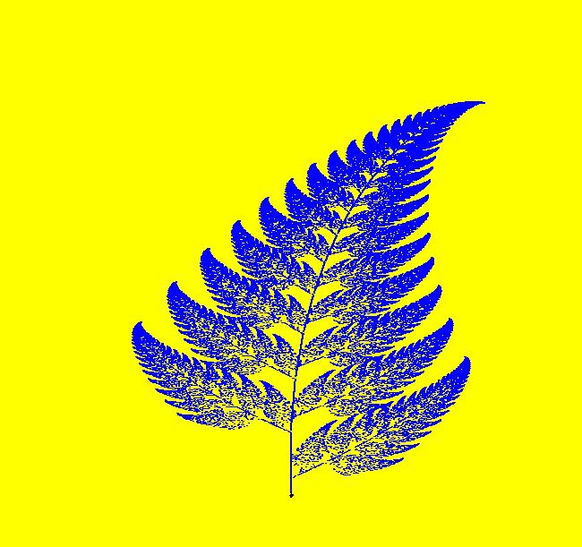
View/Sys/Gal: IMap "{Barnsley} Fern, IMap0010" in "ClassicFractals." This is a 3D IMap system consisting of four 2D linear systems that are switched On/Off at random by the z <- random(0,1) iteration. The four functions of z: A, B, C and D, act as the On/Off switches. This kind of system is, in general, called an Iterated Function System: IFS. The IMap is defined by the iterations: x <- A*0+ B*(.2*x-.26*y)+ C*(-.15*x+.28*y)+ D*(.85*x+.04*y), y <- A*.16*y+ B*(.23*x+.22*y+1.6)+ C*(.26*x+.24*y+.44)+ D*(-.04*x+.85*y+1.6), z <- random(0,1). Parameters are: a=.01; b=.08; c=.15 Functions are: A=step(z-0)-step(z-a); B=step(z-a)-step(z-b); C=step(z-b)-step(z-c); D=step(z-c)-step(z-1); The parameter values are set so that A is On 1% of the iteration time, B and C are On 7% of the iteration time and D is On 85% of the iteration time. The three parameter values: a, b and c, must be selected to partition the interval [0,1] into four segments: (0,a]+(a,b]+(b,c]+(c,1]. For each random z value in [0,1] one of the four functions is 1 and the other three are 0. Consequently the x and y iterations switch randomly between the four different linear systems as the iteration runs. The relative sizes of the partitions determine the fraction of the time each of the four linear systems is used. ICs are: (x,y,z)= (0,0,0). All ICs give the same image. The iteration consists of 110,000 steps. Try adjusting the three parameter | |||||||||||||||||||||||||||||||||||||||||||||||||||