Click on an image to go directly to a system or scroll to see the systems in this gallery.
 |
 |
 |
 |
 |
 |
 |
 |
 |
 |
 |
 |
 |
 |
 |
 |
 |
 |
 |
 |
 |
 |
 |
 |
 |
 |
 |
 |
 |
 |
 |
 |
 |
 |
 |
 |
 |
 |
 |
 |
| OdeFactory Images and Annotations | |||||||||||||||||||||||||||||||||||||||||||||||||||||||||||||||||||||
|
An OdeFactory Slide Show Click on a slide to zoom in. Click "video" to see a video. |
View/Sys/Gal: Ode " About This Gallery" in "AGFEMapExs." This gallery is a collection of 2D systems resulting from AGFs defined by two complex lines. Each complex line has 8 parameters. Consequently each AGF has 16 adjustable parameters. By varying the parameters, each complex line can generate a: center, spiral or star. For any choice of the 16 parameters the AGFs can be converted to the "dx/dt, dy/dt" form, without parameters. In this gallery, the resulting systems are designated by using "AGFv" in the system names. The parameterless AGFv systems can be made more interesting by adding a few parameters. The gallery begins with a discussion of AGFs defined by one complex line. These AGFs can produce: points, straight lines, circles, squares and spirals in various views. The last 4 systems in the gallery demonstrate connections between AGFs defined by 2 complex generators and the Mandelbrot fractals. Defining complex lines at (-a,-b) and (a,b) and setting λ2 = - λ1 will produce all of the Mandelbrot fractals. Gallery AGFs&Mandelbrot contains a detailed discussion of how to find (a,b) and λ1. Breaking the symmetry gives interesting new extensions of the Mandelbrot fractals.
|
||||||||||||||||||||||||||||||||||||||||||||||||||||||||||||||||||||
|
|
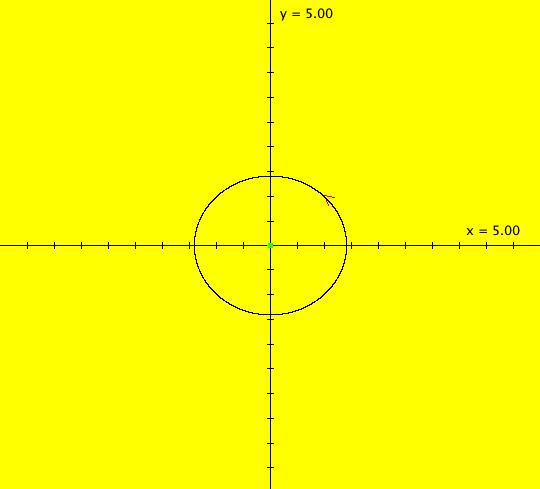
View/Sys/Gal: Ode "(0) AGF: center ccw" in "AGFEMapExs." This AGF is generated by the lines: I[1]: x+i*y = 0, λ1 = -i The degree of the RHS of the system is: 1. Complex "lines" are used in complex conjugate pairs as generators in AGFs. The other complex line in this example is conj(I[1]): x-i*y = 0. ICs: (x,y) = (1,1) re( λ1) determines the rate of the radial motion and sign(re( λ1)) determines the direction of radial motion (+ = out, - = in) im( λ1) determines the rate of the angular motion and sign(im( λ1) determines the direction of angular motion (+ = cw, - = ccw). This system has 8 parameters. If we restrict parameter changes to changes in λ only the bifurcation diagram, in the complex plane, is: real axis -> stars, complex axis -> centers, quadrants -> spirals, origin -> fixed point
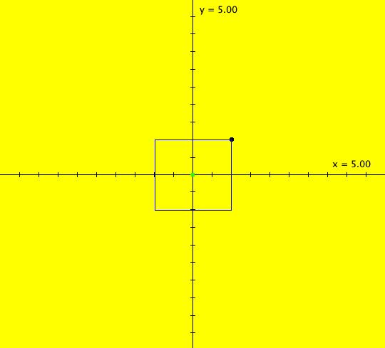
Note that the center and star states are not stable in that a small change will cause either to become a spiral. Image 1: Ode view, all trajectories are circles w/period 2* π. Image 2: IMap view, all orbits are squares w/period 4. The traditional cartesian coordinate "dx/dt, dy/dt" form of the system is: dx/dt = -y, dy/dt = x. To get to the corresponding polar coordinate form use: r' = (x*x'+y*y')/r = 0 and (no motion in radial direction) θ' = (x*y'-y*x')/r^2 = 1 (constant ccw motion in angular direction) or, in OdeFactory notation, the system is "dx/dt = 0, dy/dt = 1" in polar coordinates with ICs (x,y) = (sqrt(2),pi/4) = (1.4141,.7854)
|
|
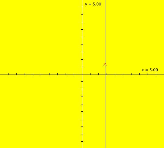
View/Sys/Gal: IMap "(0b) AGFv: center ccw, polar coordinates" in "AGFEMapExs." This system of odes is defined by the equations: dx/dt = 0, dy/dt = 1. ICs: (1.4141,.7854) Image 1: Ode view, of what was a center in cartesian coordinates polar coordinates. The circular trajectories become straight lines. Image 2: IMap view, all orbits go to the fixed point (0,1) in one iteration. Think of x as r and y as θ. "r is constant and θ increases" as expected.
|
|
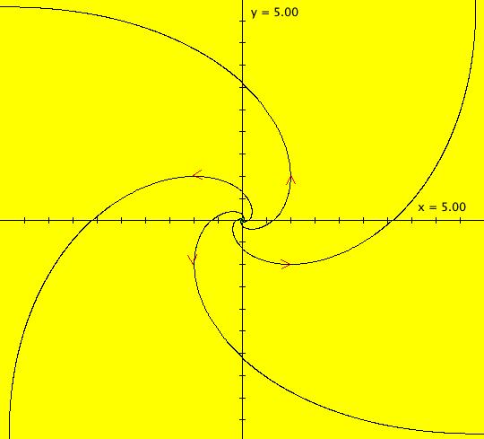
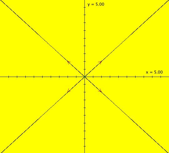
View/Sys/Gal: EMap "(0c) AGF: spiral out ccw" in "AGFEMapExs." This AGF is generated by the lines: I[1]: x+i*y = 0, λ1 = (1-i) The degree of the RHS of the system is: 1. ICs: (x,y) = (1,1) Image 1: Ode view, all trajectories are ccw spirals-out. Image 2: Ode in 3D/(t,x) view. Image 3: IMap view, all orbits are ccw spirals-out. Image 4: EMap view, zoomed in a bit, w/CT 2. The traditional cartesian coordinate "dx/dt, dy/dt" form of the system is: dx/dt = x-y, dy/dt = x+y To get to the corresponding polar coordinate form use: r' = (x*x'+y*y')/r = r and (radial motion is out) θ'= (x*y'-y*x')/r^2 = 1 (angular motion is ccw) or, in OdeFactory, notation, the system is "dx/dt = x, dy/dt = 1" in polar coordinates with ICs (x,y) = (sqrt(2),pi/4) = (1.4141,.7854)
|
|
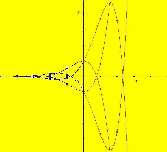
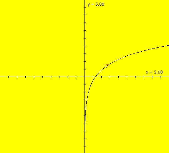
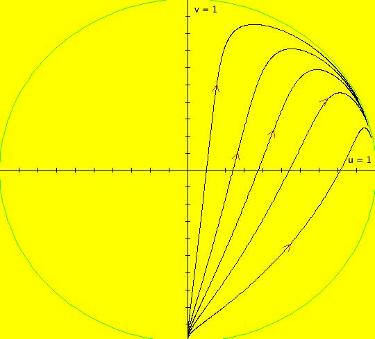
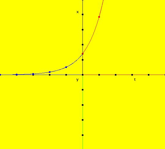
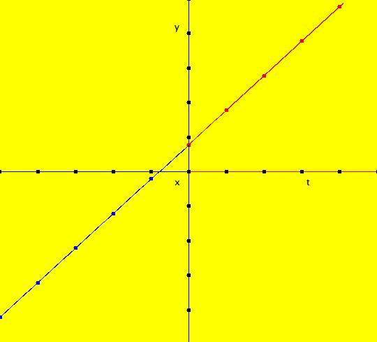
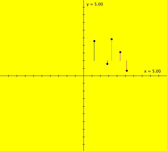
View/Sys/Gal: IMap "(0d) AGFv: spiral out ccw, polar coordinates" in "AGFEMapExs." This system of odes is defined by the equations: dx/dt = x, dy/dt = 1. ICs: (1.4141,.7854) It shows a "spiral" in polar coordinates. Spiral trajectories become x(t)= x(0)*e^t, y(t)=y(0)+1. Image 1: Ode (x,y) view. Image 2: Ode R2+ view w/fixed point at (u,v) = (1,0). Image 3: 3D/(t,x) Ode view. Image 4: 3D/(t,y) Ode view. Image 5: IMap view, all orbits go to the fixed points (x,1). Think of x as r and y as θ. "r increases as r(0)*e^t and θ increases as θ(0)+t" as expected. See the 3D/(t,x) and 3D/(t,y) views.
|
|
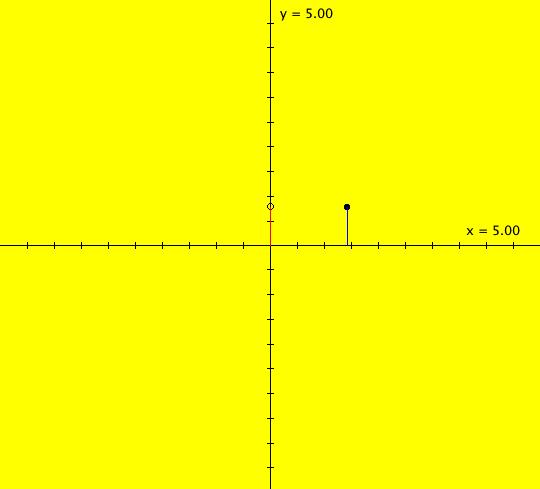
View/Sys/Gal: IMap "(0e) AGF: star out" in "AGFEMapExs." This AGF is generated by the lines: I[1]: x+i*y = 0, λ1 = 1 The degree of the RHS of the system is: 1. ICs: (x,y) = (1,1) Image 1: Ode view, all trajectories are straight lines. Image 2: IMap view w/"Show 2D IMap Orbit Sequence" on, all seeds are fixed points. The traditional cartesian coordinate "dx/dt, dy/dt" form of the system is: dx/dt = x, dy/dt = y To get to the corresponding polar coordinate form use: r' = (x*x'+y*y')/r = r and (radial motion is out) θ' = (x*y'-y*x')/r^2 = 0 (no angular motion) or, in OdeFactory notation, the system is "dx/dt = x, dy/dt = 0" in polar coordinates with ICs (x,y) = (sqrt(2),pi/4) = (1.4141,.7854)
|
|
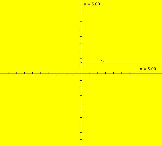
View/Sys/Gal: IMap "(0f) AGFv: star out, polar coordinates" in "AGFEMapExs." This system of odes is defined by the equations: dx/dt = x, dy/dt = 0. Ics: (1.4141,.7854) Image 1: Ode view, all trajectories are straight horizontal lines. The y axis consists of Ode fixed points. Image 2: IMap view, all seeds (x,y) go to (x,0). The x axis consists of IMap fixed points. "r increases and θ stays constant" as expected. It shows a "straight radial line" in polar coordinates. Radial trajectories in cartesian coordinates become straight lines parallel to the horizontal axis in polar coordinates. Think of x as r and y as θ. "r increases as r(0)*e^t and θ increases as θ(0)+t" as expected. See the 3D/(t,x) and 3D/(t,y) views.
|
|
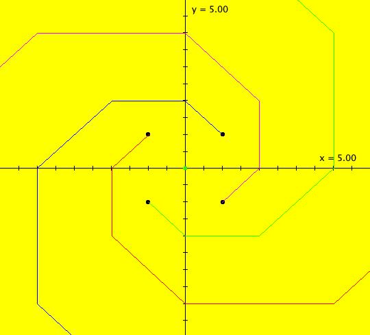
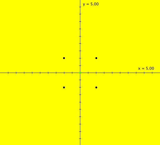
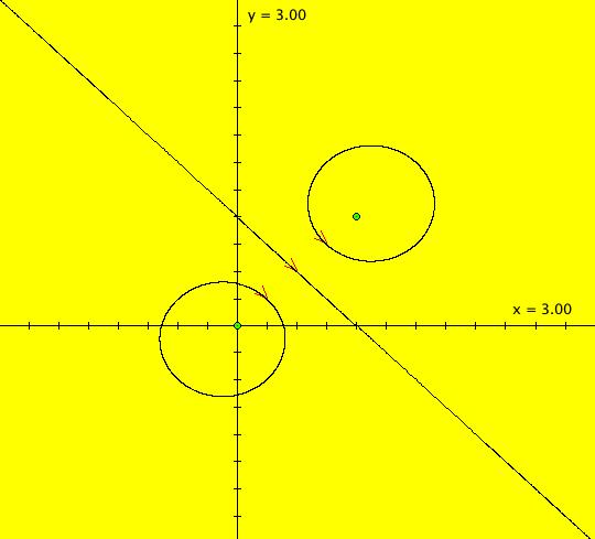
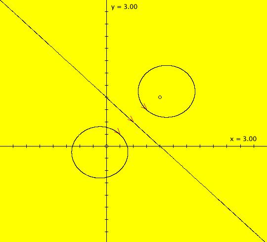
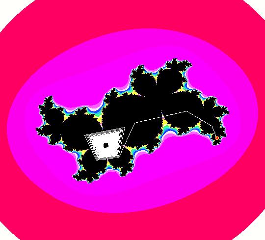
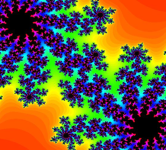
View/Sys/Gal: IMap "(1) AGF two centers" in "AGFEMapExs." This AGF is generated by the lines: I[1]: x+i*y = 0, λ1 = i I[2]: (x-1)+i*(y-1) = 0, λ2 = -i The first is a cw center at (0,0) and the second is a ccw center at (1,1). The two green dots are I[1] and I[2]. Clicking on a line opens the line's parameter controller. The degree of the RHS of the system would in general be 3 but it is reduced to 2 in this case because of symmetry. This AGF has interesting IMap and EMap views. Image 1: Ode view centered at (.5,.5). Image 2: EMap view, centered at (.5,.5) w/CT 4. This is a shifted Julia set fractal. Image 3: IMap view, zoomed in, centered at (0,0). All orbits in the Julia set's prisoner set spiral in to (0,0). All other orbits go to infinity.
|
|
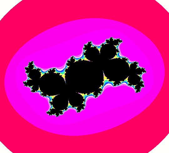
View/Sys/Gal: IMap "(1b) AGFv: two centers, p= 0, q=0" in "AGFEMapExs." This system of odes is defined by the equations: dx/dt = y+0.5*x^2-x*y-0.5*y^2+p, dy/dt = -x+0.5*x^2+x*y-0.5*y^2+q. Parameters are: p=0; q=0 It is the "dx/dt, dy/dt" form of (1) with parameters p and q added. If p+q=0 then we get two centers otherwise we get two spirals. Image 1: Ode view centered at (.5,.5). Image 2: EMap view, centered at (.5,.5) w/CT 4. This is a shifted Julia set fractal. All orbits in the prisoner set (black region) spiral in to (0,0). Image 3: IMap view, zoomed in, centered at (0,0).
|
|
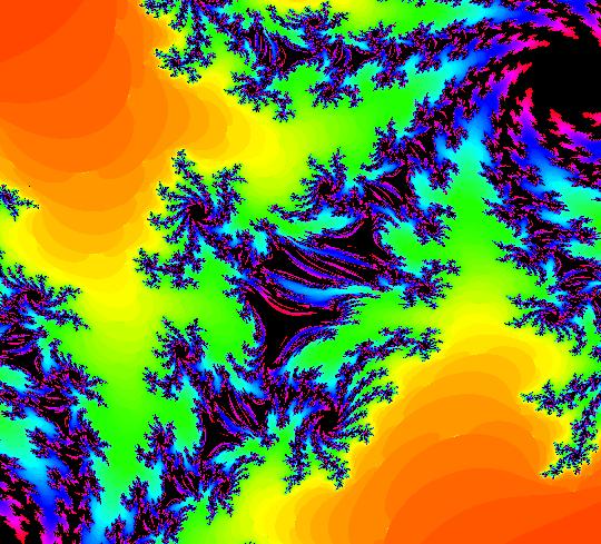
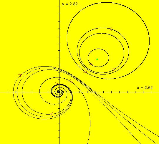
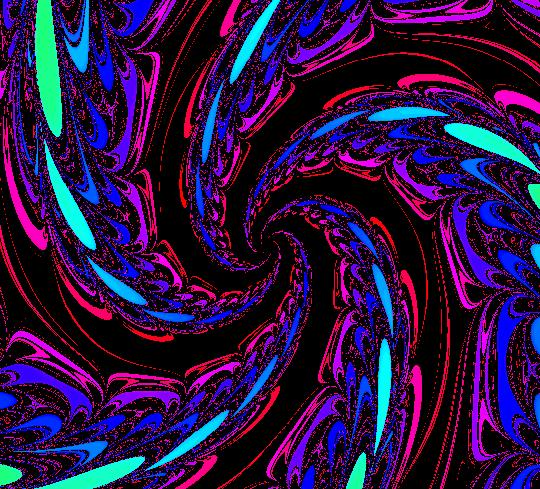
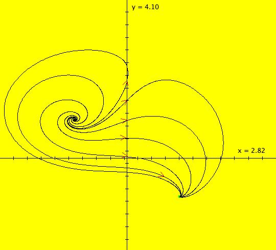
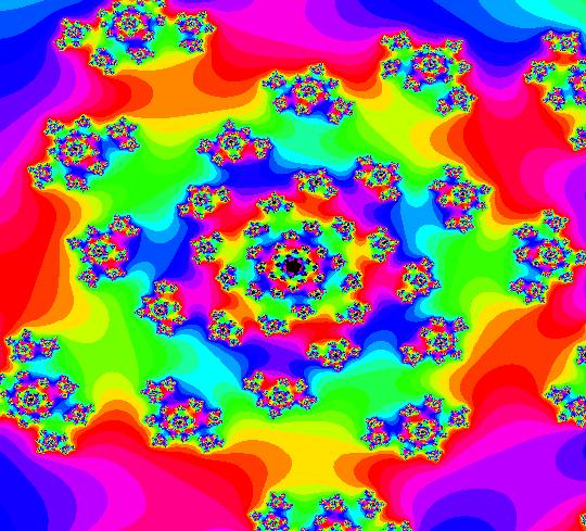
View/Sys/Gal: Ode "(2) AGF center & spiral, as EMap" in "AGFEMapExs." This AGF is generated by the lines: I[1]: x+i*y = 0, λ1 = (0.2+i), spiral I[2]: (x-1)+i*(y-1) = 0, λ2 = -i, center The degree of the RHS of the system is: 3. A center and a spiral will never produce a Julia set because the symmetry of z <- z^2+c is broken. Image 1: EMap view. The symmetry is broken here, λ2 is not quite - λ1. So this is a variation of a Julia set. Image 2: EMap view zoomed in. Image 3: Ode view. The broken symmetry is very obvious here.
|
|
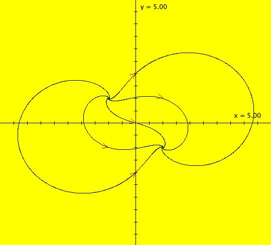
View/Sys/Gal: EMap "(3) AGF two spirals" in "AGFEMapExs." This AGF is generated by the lines: I[1]: (x+1)+i*(y-1) = 0, λ1 = (2-i) I[2]: (x-1)+i*(y+1) = 0, λ2 = (-2+i) The degree of the RHS of the system is 2 due to the symmetry of the system. Image 1: Ode view. Image 2: EMap view w/CT 5. Another Julia set.
|
|
View/Sys/Gal: Ode "(3b) AGF 2 spirals, as EMap" in "AGFEMapExs." This AGF is generated by the lines: I[1]: (x+1)+i*(y-1) = 0, λ1 = (0.5-1.2*i) I[2]: (x-1)+i*(y+1) = 0, λ2 = (-2+0.7*i) The degree of the RHS of the system is: 3. Image 1: EMap view zoomed way in. Just an interesting image. Image 2: EMap view zoomed out and centered. Not a fractal. Try other CTs. Image 3: Ode view. No symmetry.
|
|
View/Sys/Gal: EMap "(3c) AGFv two spirals with p =.80, q = -2, as EMap" in "AGFEMapExs." This system of odes is defined by the equations: dx/dt = x*(1.5*y-0.25*x)+0.25*y^2+p, dy/dt = .25*(q-3*x^2-2*x*y+3*y^2) Parameters are: p = .80; q = -2.00; This is a variation of the "dx/dt, dy/dt" form of system (3). Image 1: EMap view. Variation of a Julia set.
|
|
View/Sys/Gal: EMap "(3d) AGFv two spirals with p=.86, q=-2, as EMapCT1" in "AGFEMapExs." This system of odes is defined by the equations: dx/dt = x*(1.5*y-0.25*x)+0.25*y^2+p, dy/dt = .25*(q-3*x^2-2*x*y+3*y^2) Parameters are: p = .86; q = -2.00; Image 1: EMap view.
|
|
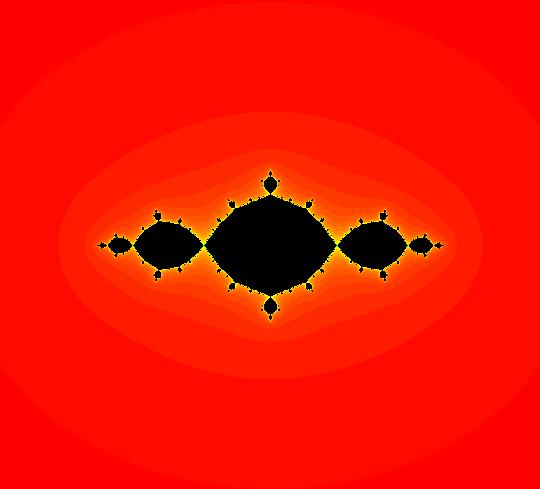
View/Sys/Gal: EMap "(4) AGF two stars, as EMap" in "AGFEMapExs." This AGF is generated by the lines: I[1]: (x+1)+i*y = 0, λ1 = -2 I[2]: (x-1)+i*y = 0, λ2 = 2 The degree of the RHS of the system would be 3 in general but for these particular parameter values it reduces to 2. Image 1: EMap view. Julia set. The system in "dx/dt, dy/dt" form, with parameters p and q added, is dx/dt = x^2-y^2+p dy/dt = 2*x*y+q p = -1, q = 0 which, for z = x+i*y, c = p+i*q is the Mandelbrot iteration z <- z^2+c. The "dx/dt, dy/dt" form of this system is discussed in system (4c).
|
|
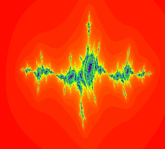
View/Sys/Gal: EMap "(4b) AGF two stars, as EMap" in "AGFEMapExs." This AGF is generated by the lines: I[1]: (1-0.01*i)*(x+1)+0.9*i*(y-0.03) = 0, λ1 = (-2.5+0.13*i) I[2]: (x-1)+i*y = 0, λ2 = 2 The degree of the RHS of the system is: 3. This is system (4) where the I[1] parameters have been changed a bit. Notice that the EMap has changed a lot. Image 1: EMap view.
|
|
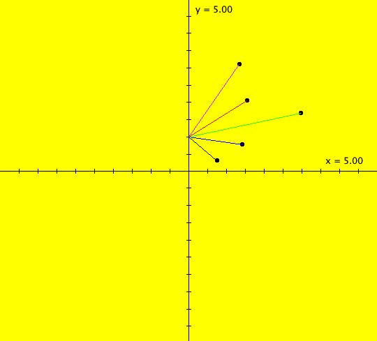
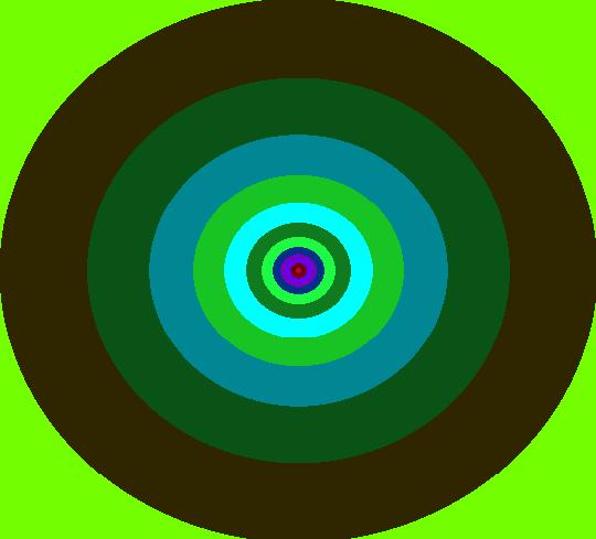
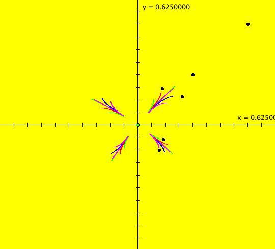
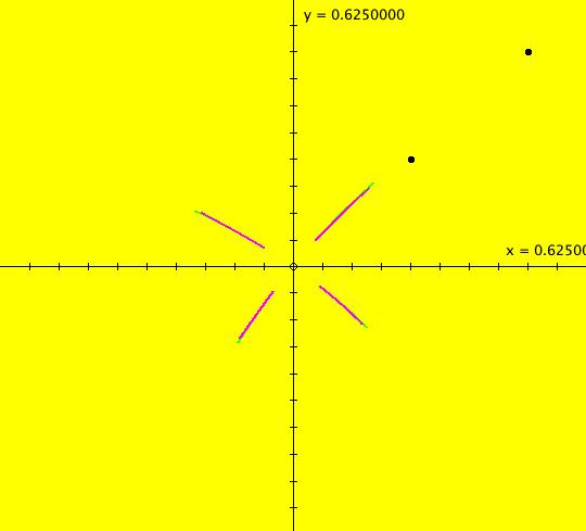
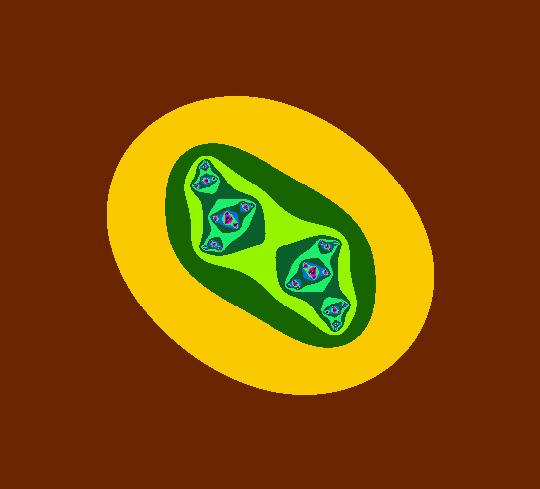
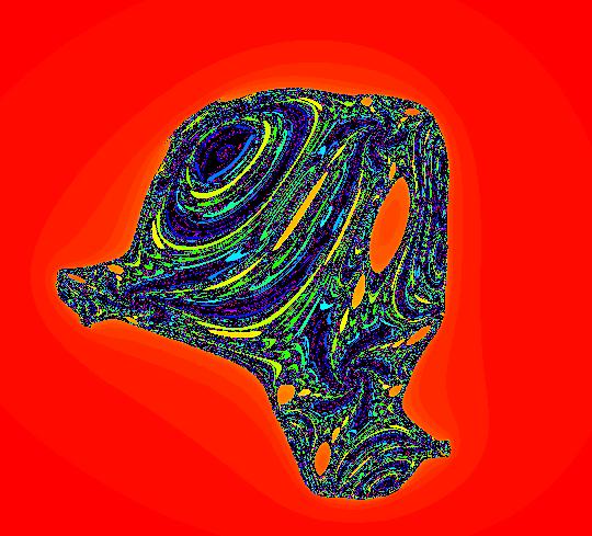
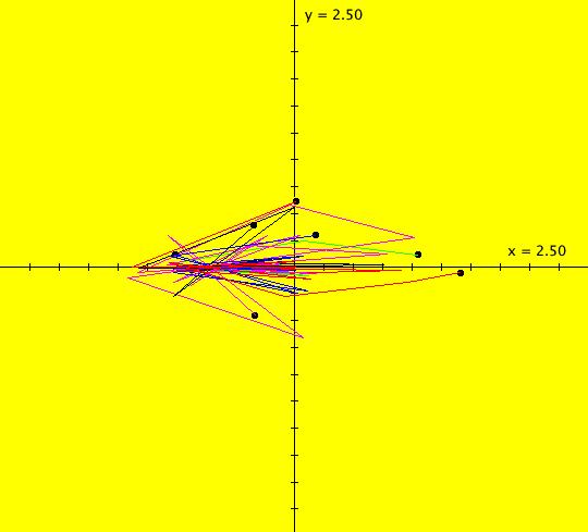
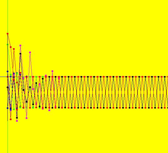
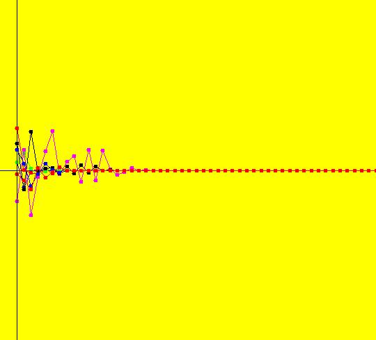
View/Sys/Gal: IMap "(4c) AGFv two stars, Mandelbrot form, as EMap" in "AGFEMapExs." This system of odes is defined by the equations: dx/dt = x^2-y^2+p, dy/dt = 2*x*y+q. Parameters are: p = -1; q = 0 Two stars iff q = 0. For p = -1, q = 0 all orbits in the prisoner set seem to have period 2. Furthermore they oscillate between x = -1 and x = 0. Image 1: EMap view. Seven orbits have been started in the prisoner set (the black region). Image 2: IMap view showing the seven orbits. Image 3: IMap 3D/(t,x) view. The oscillation in the (t,x) plane. Image 4: IMap 3D/(t,y) view. No oscillation in the (t,y) plane.
|
|
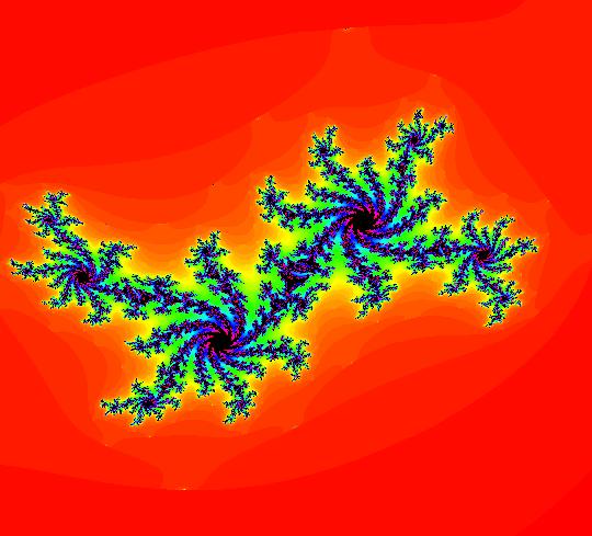
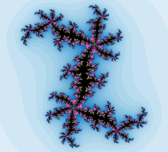
View/Sys/Gal: EMap "(4d) AGFv two stars, Mandelbrot form, p = .40; q = .35; as EMapCT3" in "AGFEMapExs." This system of odes is defined by the equations: dx/dt = x^2-y^2+p, dy/dt = 2*x*y+q Parameters are: p = .40; q = .35; Fixed points for the ode are approximately: (-.256425,.682461) and (.256425,-.682461). Image 1: IMap view. A nice Julia set.
| ||||||||||||||||||||||||||||||||||||