Click on an image to go directly to a system or scroll to see the systems in this gallery.
 |
 |
 |
 |
 |
 |
 |
 |
 |
|
|
|
 |
 |
 |
 |
 |
 |
 |
 |
 |
 |
 |
 |
 |
 |
 |
 |
 |
 |
 |
 |
 |
 |
 |
 |
 |
 |
 |
 |
 |
 |
 |
 |
 |
 |
 |
 |
 |
 |
 |
 |
 |
 |
 |
 |
 |
 |
 |
 |
 |
 |
 |
| OdeFactory Images and Annotations | |
|
An OdeFactory Slide Show Click on a slide to zoom in. Click "video" to see a video. |
View/Sys/Gal: Ode " Examples from Strogatz textbook" in "StrogatzExs." *************** Introduction *************** This gallery contains examples from the textbook "Nonlinear Dynamics and Chaos" 1994 by Steven H. Strogatz. Additional related examples, not found in the textbook, have names with page numbers followed by a letter. The Strogatz videos for the course are here. The goal is to investigate the most significant geometric features, such as: fixed points, separatrices, limit cycles, strange attractors and bifurcation diagrams - of 1D, 2D and 3D dynamical systems defined by vector fields. The systems can be viewed as Odes or as IMaps. Most of the Strogatz examples can be investigated using the math techniques presented in the textbook - however, for more complicated systems the math techniques often become to difficult to apply and computer analysis is required. In this gallery all of the examples will be studied using OdeFactory. For 1D systems with parameters, bifurcation diagrams can be found by promoting a parameter to a variable in a related 2D system. ******** Continuous vs Discrete Time ******** The logistic system is discussed in the textbook from the continuous and the discrete point of view, first, in the p. 23 example, as the continuous-time Ode: dx/dt = r*x*(1-x) (A1) and later, in the p. 357 example, as the discrete-time IMap: x <- r*x*(1-x). (A2) Since the system is a 1P1D (1 parameter, 1 dimensional) system, the bifurcation diagram for the Ode (A1) can be created using 2D Ode: dx/dt = 0, (B1) dy/dt = x*y*(1-y) and for the IMap (A2) using the 2D IMap: x <- x, (B2) y <- x*y*(1-y). Note that the motion is the same for (B1) and (B2) as it is for (A1) and (A2) so the 2D systems show the dynamics as well as the bifurcation diagrams of the 1D systems. For completeness, systems p. 23b and p. 357b have been added to the gallery. The continuous Ode view of the logistic system is not very interesting mathematically but the discrete IMap view of the system is.
|
|
|
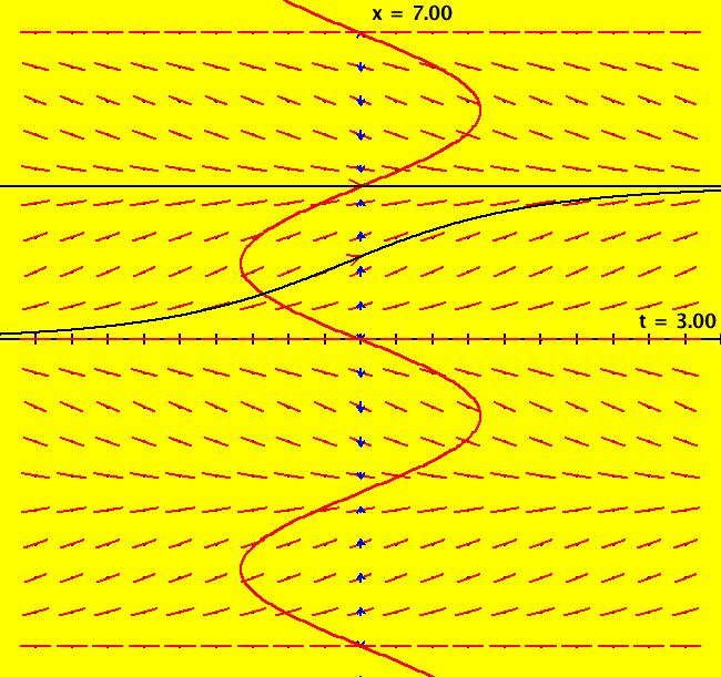
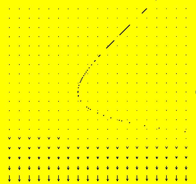
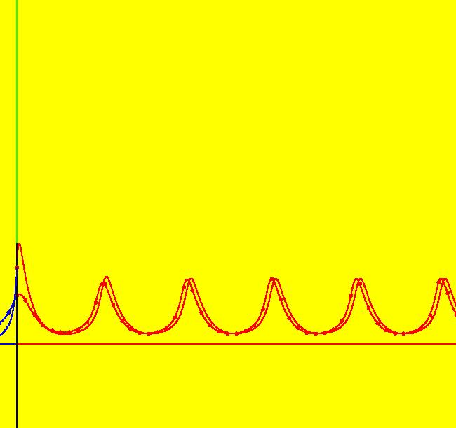
View/Sys/Gal: Ode "p. 18, fig. 2.1.3, 1D finding fixed points" in "StrogatzExs." This first ode is defined by: dx/dt = V(x) = sin(x). The motion on trajectories of the 1D Ode is in the 1D phase space (the x-axis) and the solution curves, x(t), are in the 2D extended phase space (the tx-plane). The projection of a solution curve from the extended phase space onto the phase space gives the corresponding trajectory. For 1D autonomous Ode systems we want to find: (a) the fixed points, (b) the stability of the fixed points and (c) the solution curves. Image 1: The vector field, V(x), is shown on the x axis by the blue arrows. The direction of the vector field shows the direction of the motion in the phase space. If you think of the -t axis as a +y axis, the red curve, superimposed on the extended phase space, is "y = V(x)" which provides another more detailed way to view the "vector field." Points where V(x) intersects the x-axis are the fixed points. There are no parameters so there is no bifurcation digram. To see the motion in the phase space, click the "Flow" button. The points where dx/dt = V(x) = sin(x) = 0, that is, where V(x) crosses the x axis, called the fixed points of the system, are at x = n*pi. Clicking on an IC (on an arrowhead on a solution curve) gives the asymptotic location of the fixed points associated with the solution curve. For the curved solution curve shown at IC (0,1.7): p(100.0000000000142500) = (3.1415926535897714) p(0.0000000000000000) = (1.7000000000000000) p(-100.0000000000142500) = (0.0000000000000000) so there is a stable fixed point at x = π and an unstable fixed point at x = 0. The straight line solution curve is at the (0, π) fixed point: p(100.0000000000142500) = (3.1415926535897714) p(0.0000000000000000) = (3.1415926535897714) p(-100.0000000000142500) = (3.1415926535897714). Blue arrows pointing into/out of a fixed point show the stability of the fixed point. Both arrows in => stable, both out => unstable. Analytically the sign of dv/dx at a fixed point indicates the stability of a fixed point. Open WolframAlpha (WA) by selecting "WolframAlpha" on the Help menu. If you copy/paste: sin(x) = 0 into WA you get all of the fixed points: x = n* π, n = integer. If you copy/paste: solve dx/dt = sin(x); x(0)=1.7 into WA, you get the analytic solution, when there is one, in this case: x(t) = 2*arccot(0.878478*e^(-t)) Also, copy/paste to WA: plot x(t) = 2*arccot(0.878478*e^(-t)) from t=-3 to t=3 Solution curves starting at the same x coordinate, but at different t coordinates, are translates of each other, i.e. they just differ by a phase shift. Phase shifted solution curves have the same trajectory but the motion on the trajectory start at different times.
|
|
|
View/Sys/Gal: Ode "p. 23, fig. 2.3.4, 1D logistic equation" in "StrogatzExs." This ode is defined by the equation: dx/dt = r*x*(1-x/k) for k ≠ 0 in the (t,x) coordinate system. Parameters are: r=1; k=1 The presence of parameters r and k make this a family of odes. Image 1: The slope field, vector field, vector field, V(x) = r*x*(1-x/k), and sample x(t) solution curves. Click the "Flow" button to see the motion. If you vary the control parameters r and k and watch what happens to V(x) and the fixed points. Notice that r changes the magnitude of the vector field (scales time) and k changes the location of the fixed points. Note: changing r and/or k gives you a new system. You can get back to the original system by reselecting the system in the list of systems in the gallery. Use WA to find the closed form solution: x(t) = (k e^(c_1 k+r t))/(e^(c_1 k+r t)-1). Note: WA notation uses a space for multiplication and can have an underscore in a parameter name, for example the c_1. Copy/paste the following into WA to find the fixed points of the system: solve 0 = r*x*(1-x/k) for x. Of course the solutions to dx/dt = 0 are obvious for this example (x = 0 and x = k) but the WA syntax works for more difficult examples. OdeFactory computes the asymptotic values for the fixed points as: p(100.0500000000142800) = (0.9999999999999944) p(0.0000000000000000) = (0.5000000000000000) p(-100.0500000000142800) = (0.0000000000000000) To see more samples of WA syntax select "WolframAlpha Syntax" on the Help menu.
|
|
|
View/Sys/Gal: Ode "p. 23b 2D bifurcation diagram for logistic equation" in "StrogatzExs." This system of odes is defined by the equations: dx/dt = 0, (B) dy/dt = x*y*(1-y/k) for k ≠ 0. Parameter r was promoted to variable x. Turn the colored V fld on. Image 1: This is the bifurcation diagram for the 2P1D Ode system: dx/dt = r*x*(1-x/k) for k ≠ 0. (A) Parameter r in (A), called x in (B), time-scales the vertical motion. To see this time-scaling try the Flow button. Try promoting k instead of r.
|
|
|
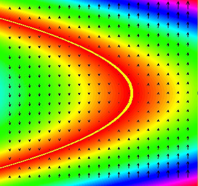
View/Sys/Gal: Ode "p. 45, fig. 3.1.1, 1D system, dx/dt = r+x^2" in "StrogatzExs." This ode is defined by the equation: dx/dt = r+x^2 (A) Parameters are: r=-1 Image 1: The slope field, vector field, and sample x(t) solution curves. For r = -1, the fixed points are at x = +-1. The fixed point at x = -1 is a sink (the flow on the x axis is "into" the fixed point) and the fixed point at x = 1 is a source (the flow is "out of" the fixed point). Click the "Flow" button and start some random trajectories to see the motion on the x axis generated by the vector field. As r increases, the fixed points come together and vanish at r = 0. To see this happen, click the "Adj Params" button and increase r. For r = 0 we have an example of a "saddle-node bifurcation." The flow at the (0,0) fixed point is out on the +x axis and in on the -x axis. As r goes negative the (0,0) fixed point bifurcates (splits) into two fixed points. The next system, shown in figure 3.1.4 on page 46 of Strogatz, shows the bifurcation diagram for this system. It is generated in OdeFactory by defining the related 2D system where the vertical y axis plays the role of x in dx/dt = r+x^2 and the horizontal axis x plays the role of the bifurcation parameter r. The related 2D "bifurcation diagram" system is: dx/dt = a, (B) dy/dt = x+y^2, a = .05 Setting an IC for x in system (B) corresponds to selecting a value for r in the system (A). Since r is a constant for each version of system (A), dx/dt should be set to 0 in system (B). However, with "V On" in (B) if we instead set dx/dt = a = .05, OdeFactory will draw the bifurcation diagram, using system (B), showing the approximate bifurcation curve x+y^2 = 0 as the x-nullcline. With a = 0 the bifurcation curve is shown as the dotted line of fixed points of the system (B). Sometimes the nullcline view is best, sometimes the fixed points view is better.
|
|
|
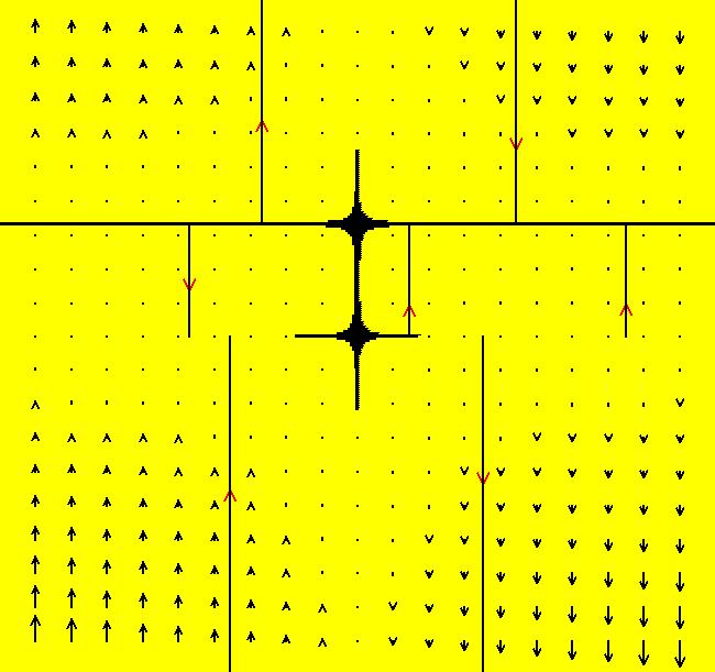
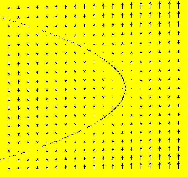
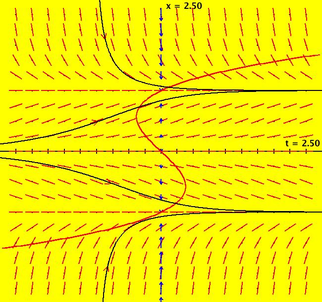
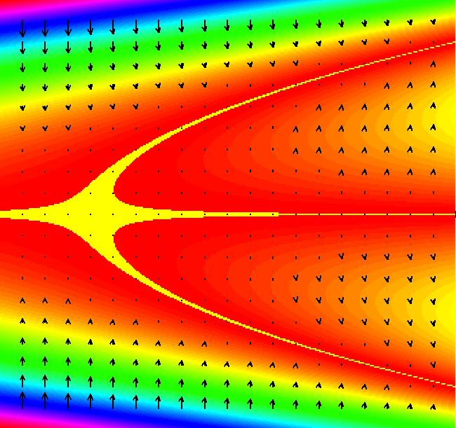
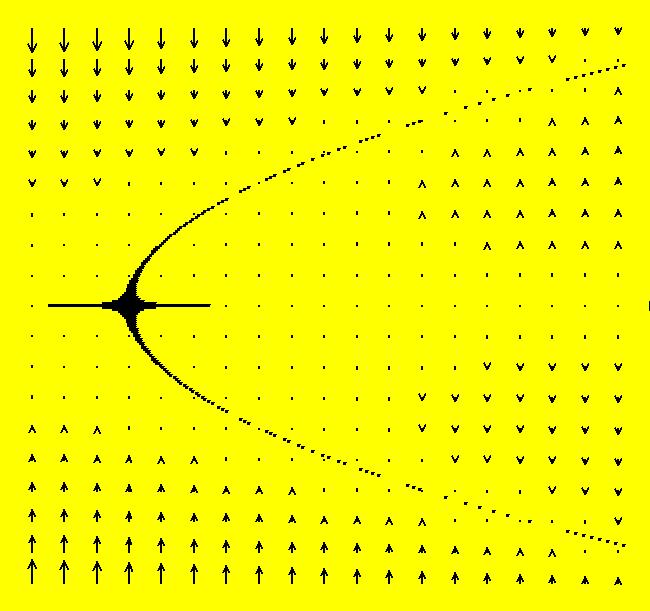
View/Sys/Gal: Ode "p. 46, fig. 3.1.4, 2D bifurcation diagram for dx/dt = r+x^2 " in "StrogatzExs." To create the bifurcation diagram of a one parameter 1D system of odes: dx/dt = f(r,x) (A) promote the parameter of the 1D system (A) to the variable x in the 2D companion system (B): dx/dt = a, (B) dy/dt = f(x,y), a = .05 or 0. Parameters can be thought of as fixed "constants" during the motion or as changeable "variables" before the motion. Changing the parameter values generally results in qualitatively different kinds of motion. Bifurcation diagrams show all of the possible different kinds of motion generated by a system when all possible different parameter values are used. Generally bifurcation diagrams are static maps of the regions in the parameter space that correspond to topologically different kinds of motion. However, for 1P1D systems, OdeFactory can animate the corresponding 2D bifurcation diagrams. Turn the colored V fld on. If a = .05 the yellow x-nullcline is the approximate bifurcation curve of (A). If a = 0 the fixed point dots of (B) are on the bifurcation curve of (A). Aside: The OdeFactory code for "Show Colored Vector Field w/Nullclines" uses yellow for points near nullclines. When a = 0, dx/dt = 0 for all (x,y) so all points are yellow and the "Colored Vector Field" is all yellow. For this particular system (B), with a = 0, the fixed points are on x+y^2 = 0 which is the parabola: y = +-sqrt(-x) for x <= 0. The black dots form the bifurcation curve of system (A). The vector field of system (B) shows the direction of motion on the x axis for system (A) for various r values, i.e. x values for system (B). Image 1: When a = .05 the bifurcation curve for dx/dt = r+x^2 is shown by the yellow x-nullcline of system (B). Image 2: When a = 0 the bifurcation curve for dx/dt = r+x^2 is shown by the fixed points of system (B). Try the Flow button to see the motion of the 1D system in the 2D bifurcation diagram.
|
|
|
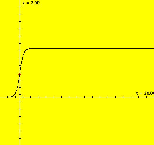
View/Sys/Gal: Ode "p. 47, fig. 3.1.6, 1D system, dx/dt = r-x-e^(-x)" in "StrogatzExs." This ode is defined by the equation: dx/dt = r-x-e^(-x) Parameters are: r = 2.00; Image 1: The slope field, vector field, and sample x(t) solution curves. For r > 1 there are two fixed points and the flow on the x axis, starting from large x values, is down, then up, then down again. For r = 1 there is one fixed point at x = 0. The flow is into the fixed point for x > 0 and out of the fixed point for x < 0. The fixed point is semi-stable. For r < 1 there is no fixed point and the flow is all down. Adjust the control parameter r and watch what happens.
|
|
|
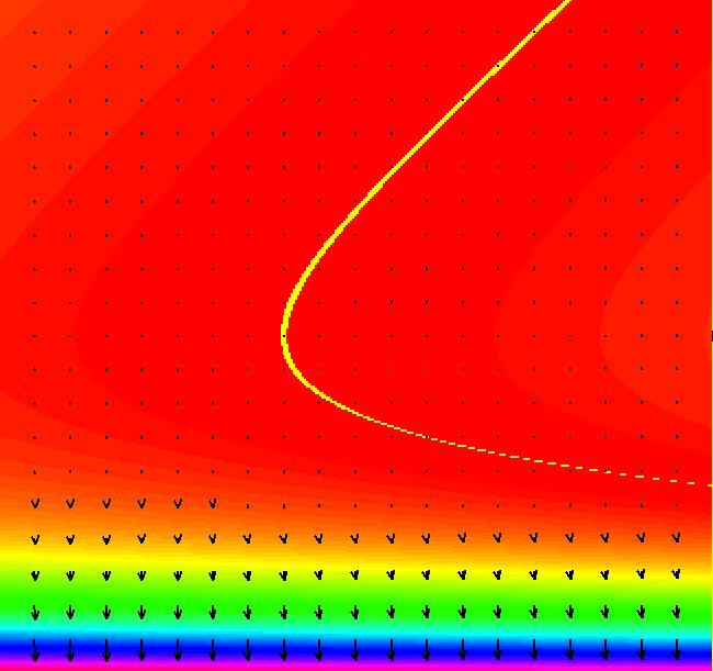
View/Sys/Gal: Ode "p. 47b, fig. 3.1.6, 2D bifurcation diagram for dx/dt = r-x-e^(-x)" in "StrogatzExs." This system of odes is defined by the equations: dx/dt = a, dy/dt = x-y-e^(-y). Parameters are: a=.05 Turn the colored V fld on. Image 1: The yellow curve is the a = .05 bifurcation curve for dx/dt = r-x-e^(-x). Image 2: The dotted line is the a = 0 bifurcation curve for dx/dt = r-x-e^(-x). Try the Flow button.
|
|
|
View/Sys/Gal: Ode "p. 50, fig. 3.2.2, 2D transcritical bifurcation for dx/dt = r*x-x^2" in "StrogatzExs." This system of odes is defined by the equations: dx/dt = a, dy/dt = x*y-y^2. Parameters are: a = .0500; By observation, the bifurcation curves are just: y = 0 and y = x. Turn the colored V fld on. Image 1: The a = .05 view. Image 2: The a = 0 view. Neither view gives a very good image of these particular bifurcation curves.
|
|
|
View/Sys/Gal: Ode "p. 56, 1D system, dx/dt = r*x-x^3" in "StrogatzExs." This ode is defined by the equation: dx/dt = r*x-x^3 in the (t,x) coordinate system. Parameters are: r=1 Image 1: The slope field, vector field, and sample x(t) solution curves.
|
|
|
View/Sys/Gal: Ode "p. 56, fig. 3.4.2, 2D a pitchfork bifurcation for dx/dt = r*x-x^3" in "StrogatzExs." This system of odes is defined by the equations: dx/dt = a, dy/dt = x*y-y^3. Parameters are: a = .05 Turn the colored V fld on. Image 1: The pitchfork bifurcation diagram for system dx/dt = r*x-x^3 with a = .05. Image 2: The pitchfork bifurcation diagram for system dx/dt = r*x-x^3 with a = 0.
|
|
|
View/Sys/Gal: Ode "p. 56b, fig. 3.4.2, 2D a pitchfork bifurcation curves from H=x*y-y^3" in "StrogatzExs." This system of odes is defined by the equations: dx/dt = (a*(x-3*y^2)), (C) dy/dt = -(a*(y)). Parameters are: a = 1; Functions are: H=x*y-y^3 The 1D system is: dx/dt = r*x-x^3. (A) The corresponding 2D bifurcation diagram system is: dx/dt = 0, (B) dy/dt = x*y-y^3. The bifurcation curves for the 1D system are: x*y-y^3 = 0 => y = 0 and y = +-sqrt(x), x >= 0 which are the red H = 0 curves for the quasi-Hamiltonian system generated by OdeFactory. The quasi-Hamiltonian system (C) is not the corresponding 2D bifurcation diagram system (B). It gives a nice image of (A)'s bifurcation curve(s) but does not give (A)'s flow direction. Using WA on "plot x*y-y^3=0" gives the same pitchfork curves. Image 1: The pitchfork bifurcation curves for dx/dt = r*x-x^3 where the x-axis plays the role of "r."
|
|
|
View/Sys/Gal: Ode "p. 69, dx/dt = h+x*(r-x^2), imperfection parameter h, 2P1D system" in "StrogatzExs." This ode is defined by the equation: dx/dt = h+x*(r-x^2). Parameters are: h=0; r=1 If h = 0 the vector field V(r,x) = x*(r-x^2) is symmetric about the t axis V(r,-x) = -V(r,x). If h ≠ 0 the symmetry is broken. Image 1: The slope field, vector field, and sample x(t) solution curves.
|
|
|
View/Sys/Gal: Ode "p. 71, fig. 3.6.3, bifurcation diagram for dx/dt = h+x*(r-x^2)" in "StrogatzExs." This system of odes is defined by the equations: dx/dt = 0, (B) dy/dt = h+y*(x-y^2). Parameters are: h = .1 Parameter r got promoted to variable x, h remains a parameter. It gives the bifurcation diagram for the 2P1D system: dx/dt = h+x*(r-x^2). (A) In system (B) x plays the role of r in (A). Parameter "a" in (B) is used to toggle the x-nullcline on/off in (B). Parameter h in (A) and (B) is used to toggle between figs. 3.6.3 (a) and (b). Turn the colored vector field on. Image 1: h = .1, fig. 3.6.3 (b) Image 2: h = 0, fig. 3.6.3 (a)
|
|
|
View/Sys/Gal: Ode "p. 72, fig. 3.6.3, bifurcation diagram for dx/dt = h+x*(r-x^2) ver 2" in "StrogatzExs." This system of odes is defined by the equations: dx/dt = 0, dy/dt = x+y*(r-y^2). Parameters are: r=1 Parameter h got promoted to variable x, r remains a parameter. Turn the colored V fld on. Image 1: This is a cross-section view of the 3D surface in fig. 3.6.4 (b) and fig. 3.6.5 p. 72 of the textbook. The (h,x,r) axes in the textbook are the (x,y,t) axes in OdeFactory.
|
|
|
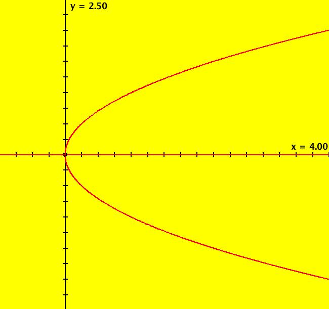
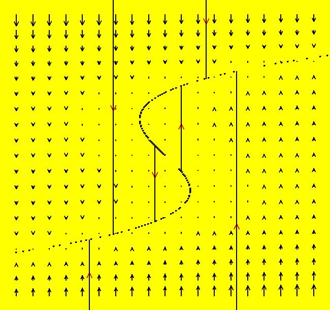
View/Sys/Gal: Ode "p. 77, fig. 3.7.4, dx/dt = r*x*(1-x/k)-x^2/(1+x^2), the 2P1D system" in "StrogatzExs." This ode is defined by the equation: dx/dt = r*x*(1-x/k)-x^2/(1+x^2) in the (t,x) coordinate system. Parameters are: r=.4; k=10 Image 1: p. 77, fig. 3.7.4 in the textbook rotated 90 degrees ccw. If you click on the arrow-heads, you will find that for r = .4, k = 10 the fxpts are at about: x = 0, .46, 3.69, 5.84 For this 2P1D system, the bifurcation space is the 2D (k,r) plane.
|
|
|
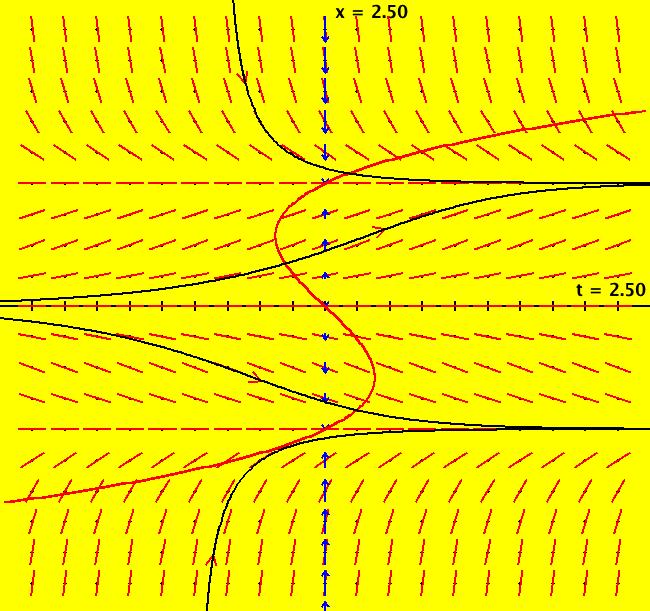
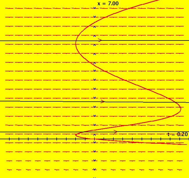
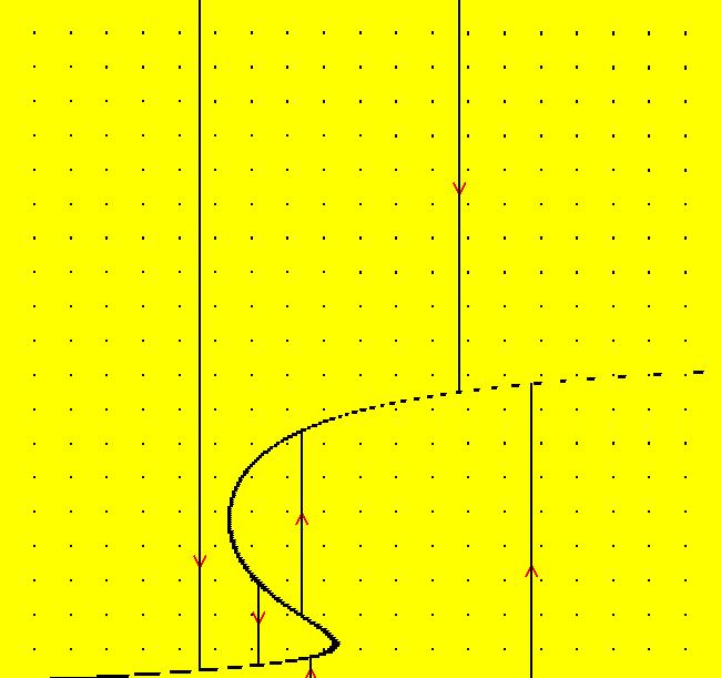
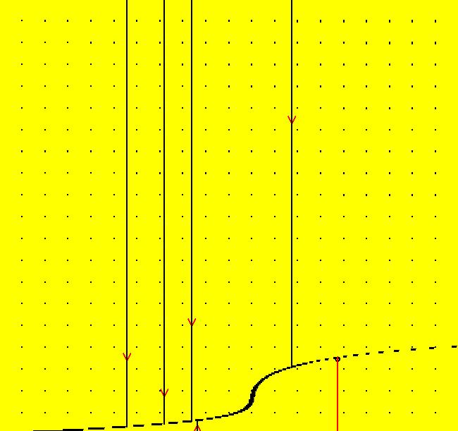
View/Sys/Gal: Ode "p. 78, fig. 3.7.6, bifurcation diagram for 2P1D system" in "StrogatzExs." This system of odes is defined by the equations: dx/dt = a, dy/dt = x*y*(1-y/k)-y^2/(1+y^2). Parameters are: a = .0000; k = 10.0000; The r parameter got promoted to x, y is the "x" from the 2P1D system and parameter k remains a parameter. Turn the colored V fld on. Image 1: This is the cross-section view of the 3D surface in fig. 3.7.6 p. 78 of the textbook. The (r,x,k) axes in the textbook are the (x,y,t) axes in OdeFactory. The projections of the right most point and the left most point of the S shaped curve onto the (k,r) plane, as a function of decreasing k, gives fig. 3.7.5 in the textbook. Image 2: For k about 5, the right most point and the left most point of the S shaped curve converge at about x = "r" = .66 as shown in fig. 3.7.5 in the textbook.
|
|
|
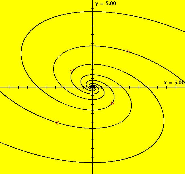
View/Sys/Gal: Ode "p. 126, 130, 134, fig. 5.2.8, 2D linear systems" in "StrogatzExs." This system of odes is defined by the equations: dx/dt = a*x+b*y, dy/dt = c*x+d*y Parameters are: a=1; b = 2; c = -1; d = 0 Image 1: A spiral-out cw system. Adjust the control parameters to see what you get. Set b = c = 0, d = -1, then set a < -1, a = -1, -1 < a < 0, a = 0 and a > 0. Let A be the coefficient matrix: {{a,b},{c,d}} so: tr(A) = a+d, det(A) = a*d-b*c. If tr(A)^2 < 4*det(A)^2 the eigenvalues of A are complex and the trajectories are ellipses when tr(A)=0 and spirals-out when tr(A)>0. Select values for a, b, c and d to get ellipses and spirals. When are the ellipses actually circles? When is the flow clockwise cw? One solution is to: set a = d = 0, then let b*c < 0 to get ellipses, and let b = -c to get circles. If b > 0 then the flow is cw. One way to get spirals, cw and out, is to set a > 0, d = 0, b*c < 0 and b > 0. The bifurcation diagram for this system is best described in the 2-parameter (det(A),tr(A)) plane. See Strogatz, p. 137, fig. 5.2.8, or most any ODE/Linear Algebra textbook, for details. Note that for 2D nonlinear systems there are no general classification schemes. Finally, in the EMap view, most linear systems produce fractals. Go to the EMap view and vary the parameters and the color tables.
|
|
|
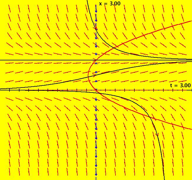
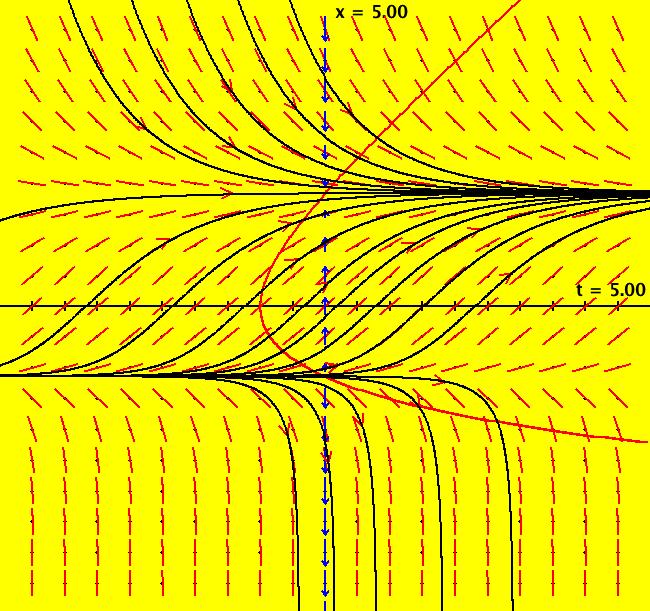
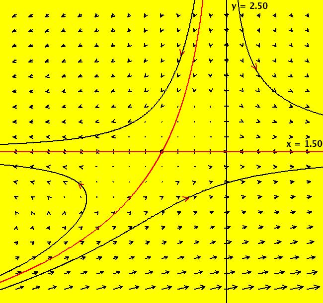
View/Sys/Gal: Ode "p. 148, fig. 6.1.4 nullclines and separatrix system of (x+e^(-y),-y)" in "StrogatzExs." This system of odes is defined by the equations: dx/dt = x+e^(-y), dy/dt = -y. Turn the colored V fld on. Image 1: The nullclines are in yellow, the separatrix system is in red. Nullclines intersect at the fixed point.
|
|
|
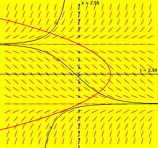
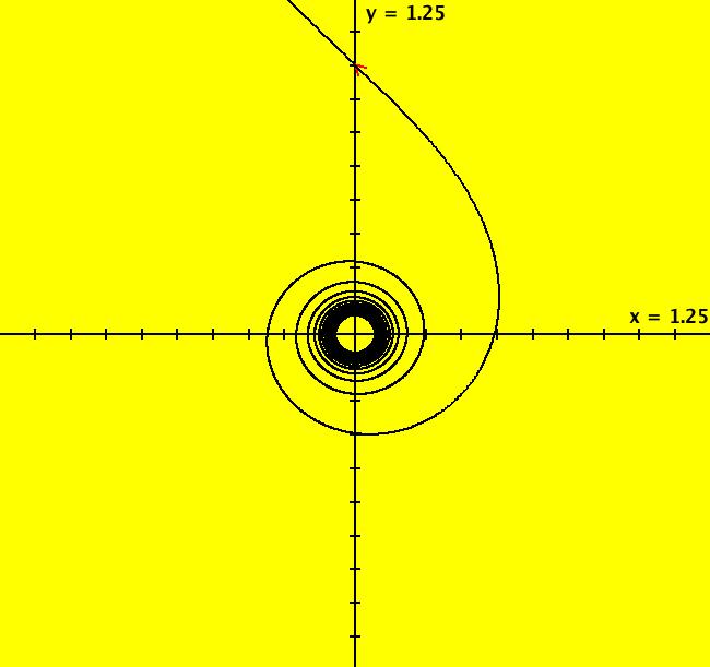
View/Sys/Gal: Ode "p. 154, fig. 6.3.2, center at (0,0) only if a = 0" in "StrogatzExs." This system of odes is defined by the equations: dx/dt = -y+a*x*(x^2+y^2), (A) dy/dt = x+a*y*(x^2+y^2) Parameters are: a=1 Linearizing system (A) at the fixed point (0,0) gives system (B): dx/dt = -y, (B) dy/dt = x for all "a." We might expect that systems (A) and (B) have similar flows near (0,0) but for (B) the origin is a center (ccw circles) and for (A) it is a center iff a = 0. So - linearizing a nonlinear system at a fixed point need not tell us much about the nonlinear system near the fixed point. Image 1: A typical a ≠ 0 case for nonlinear system (A). Adjust the control parameter "a" and observe what happens.
|
|
|
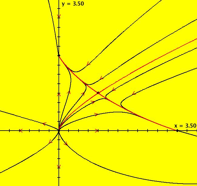
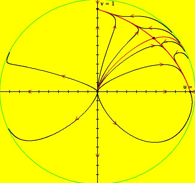
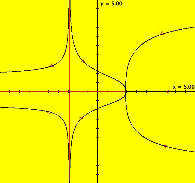
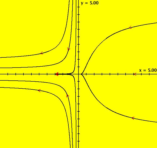
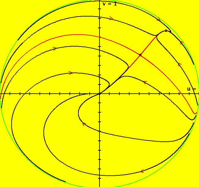
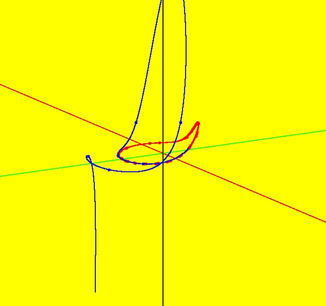
View/Sys/Gal: Ode "p. 158, fig. 6.4.7, rabbits vs sheep" in "StrogatzExs." This system of odes is defined by the equations: dx/dt = x*(3-x-2*y), dy/dt = y*(2-x-y) Copy/paste 0 = x*(3-x-2*y), 0 = y*(2-x-y) into WA to find the fixed points. x = 0, y = 2 x = 1, y = 1 x = 3, y = 0 x = 0, y = 0 Note: of course you can find these by inspection but see what WA gives you so you can use WA on harder problems. Next, evaluate the Jacobian at each fixed point using WA on: evaluate D[{x*(3-x-2*y),y*(2-x-y)},{{x,y}}] at x=0, y=0 then on evaluate D[{x*(3-x-2*y),y*(2-x-y)},{{x,y}}] at x=0, y=2 then on evaluate D[{x*(3-x-2*y),y*(2-x-y)},{{x,y}}] at x=3, y=0 then on evaluate D[{x*(3-x-2*y),y*(2-x-y)},{{x,y}}] at x=1, y=1 Finally, draw fig. 6.4.7, p. 158 of Strogatz as follows: Right click in the graphics area and enter the fixed point values. A small circle indicates that a point is a fixed point. After you have entered all four fixed points, click the t button just below the graphics area to get into the 3D view. In the 3D view, click in the graphics area to bring up the orientation controller. Change the second angle (pitch) from 15 to 45. The (x,y) plane is defined by the green and black axes. The red axis is the time axis. The +t part of the fixed point solutions are the red lines parallel to the t axis, the -t parts are in blue. The dots are one t unit apart. Deselect the t button to return to the phase plane (2D) view. To draw the (red) separatrices at (1,1), place the cursor at (1,1), hold the shift key down, then move the cursor a bit. Another way to do this is to start solutions at (1,1.0001) and (1,.9999). Values for rabbits and sheep are greater than or equal to 0 but mathematically the system is defined for all of R2 so the x and y axes are also separatrices. Try the R2+ view to see what is happening at infinity. Image 1: Rabbits and sheep system with separatrices. Image 2: R2+ view of the same system.
|
|
|
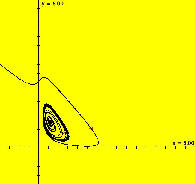
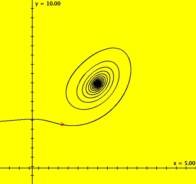
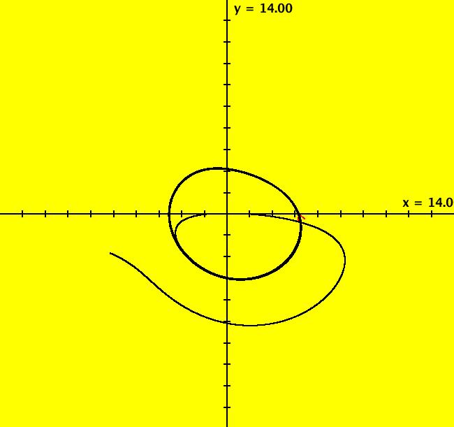
View/Sys/Gal: Ode "p. 209, fig. 7.3.8, glycolysis model" in "StrogatzExs." This system of odes is defined by the equations: dx/dt = -x+.08*y+x^2*y, dy/dt = .6-.08*y-x^2*y To see the motion defined by the vector field, click the Flow button. Copy/paste 0 = -x+.08*y+x^2*y, 0 = .6-.08*y-x^2*y into WA to find the approximate fixed point: x = .6, y = .36364 Image 1: A stable limit cycle about a fixed point. To find the approximate period of the periodic orbit extend a trajectory to +t about 5000 then use the +t end of the orbit to start a new orbit. If you select "Show Approximate Period" you get 9.62. Image 2: The 3D/(t,x) view of the limit cycle. hMin = 100, hMax = 119.62 shows two cycles on the limit cycle. How sensitive is the system to the .08 and the .6? Define a new system with parameters c = .08 and d = .6. See what happens as you adjust c and d.
|
|
|
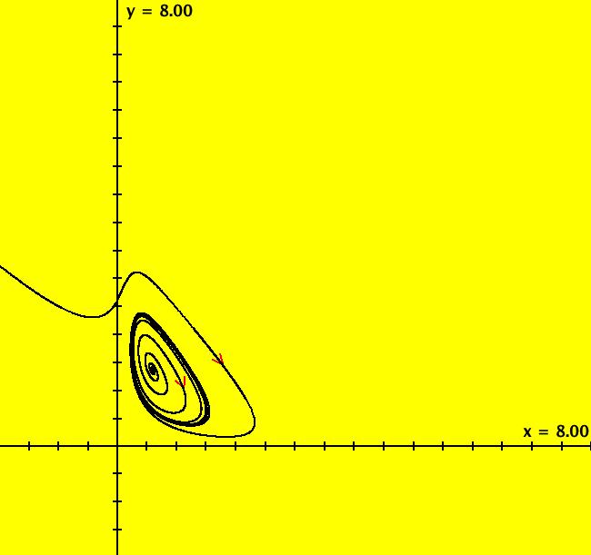
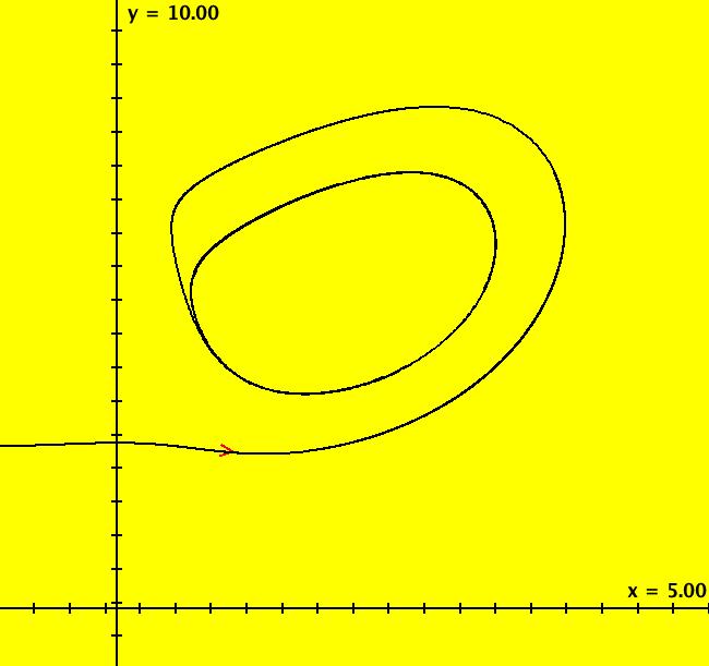
View/Sys/Gal: Ode "p. 209b, glycolysis model, c=.08; d=.6" in "StrogatzExs." This system of odes is defined by the equations: dx/dt = -x+c*y+x^2*y, dy/dt = d-c*y-x^2*y. Parameters are: c=.08; d=.6 Image 1: The inner trajectory spirals out to a limit cycle and the outer orbit spirals in to the same limit cycle. Set hMax = 50 then get into the 3D/(t,x) to see another view of the limit cycle. Image 2: 3D/(t,x), c = .08, d = .6 Vary c and d to see what happens to the limit cycle.
|
|
|
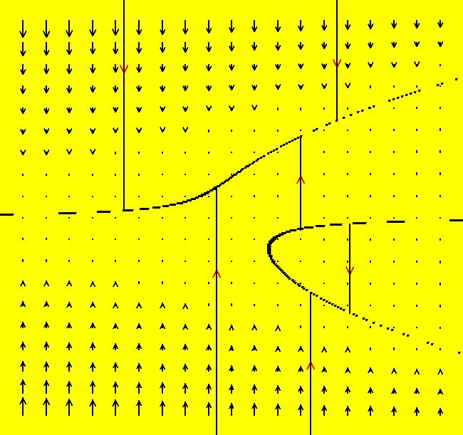
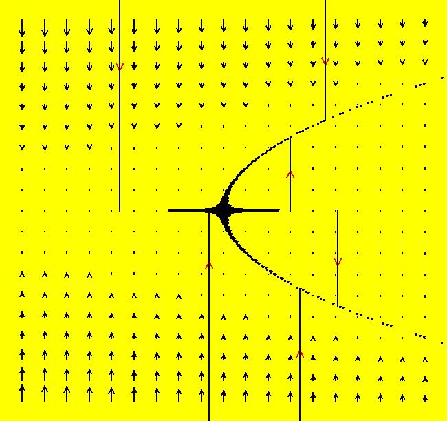
View/Sys/Gal: Ode "p. 242, fig. 8.1.1, a saddle-node bifurcation" in "StrogatzExs." This system of odes is defined by the equations: dx/dt = b-x^2, (A1) dy/dt = -y (A2) Parameters are: b = 2.10; This is an uncoupled 2D system consisting of two simple 1D systems: (A1) and (A2). (A1) has fixed points at x = +-sqrt(b) for b >= 0. The positive fixed point is stable, the negative one is unstable. (A2) has a single stable fixed point at y = 0. The separatrix system for the 2D system consists of the four red line segments plus the x axis for x > sqrt(b). For b > 0 the negative fixed point is a saddle and the positive one is a node. Note: "saddle" and "node" are terms used to describe 2D fixed points. As b decreases to 0 the two fixed points come together and vanish, or as b increases to 0 the a fixed point is born and bifurcates (splits) into two fixed points. Try adjusting the control parameter. It seems that the b > 0 part of figure 8.1.1 in the Strogatz book may be wrong. Check it out. Image 1: b > 0, fxpts at x = +-sqrt(b), y = 0 Image 2: b = 0, fxpt at x = 0, y = 0 Image 3: b < 0, no fxpts
|
|
|
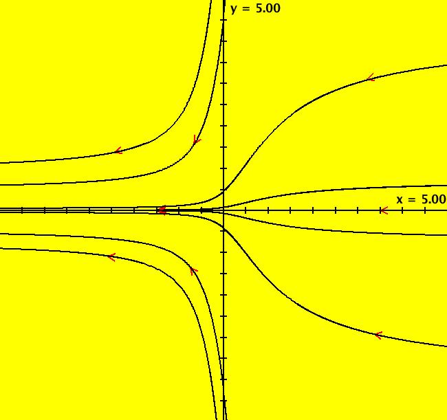
View/Sys/Gal: Ode "p. 245, fig. 8.1.5, genetic control system" in "StrogatzExs." This system of odes is defined by the equations: dx/dt = -a*x+y, dy/dt = x^2/(1+x^2)-b*y Parameters are: a=1; b=.4 Critical points are at: (0,0) and about (.5,.5) and (2,2). The nullclines are: x-nullcline: y = a*x, y-nullcline: y = x^2/(b*(1+x^2)). Turn the colored V fld on. Image 1: The nullclines and the fixed points at the intersections of the nullclines. Image 2: R2+ view of separatrix system. Adjust the control parameters.
|
|
|
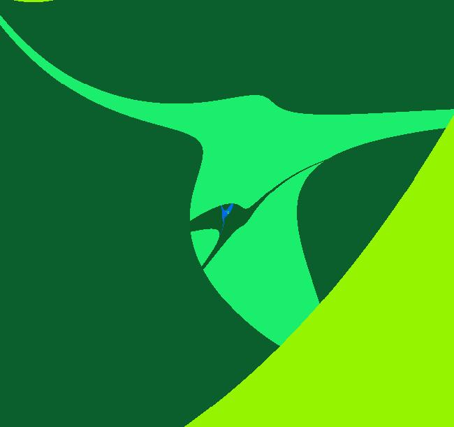
View/Sys/Gal: EMap "p. 245b, EMapCT9 art image" in "StrogatzExs." This iteration is defined by: x <- -a*x+y, y <- x^2/(1+x^2)-b*y. Parameters are: a = 1.1000; b = .5200; EMap CT: 9 Image 1: Just an interesting EMap art image.
|
|
|
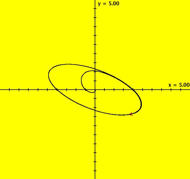
View/Sys/Gal: Ode "p. 254, fig. 8.2.6, Hopf bifurcation at (0,0)" in "StrogatzExs." This system of odes is defined by the equations: dx/dt = a*x-y+x*y^2, dy/dt = x+a*y+y^3 Parameters are: a = -1; Vary parameter "a" to see what happens. Toggle to the EMap view then adjust "a" to -0.7 and zoom in a few times. Try some different color maps. Image 1: Ode view, -t limit cycle. Image 2: EMapCT2 view, a = -.7 zoomed in. Welcome to interactive algorithm-based abstract art!
|
|
|
View/Sys/Gal: Ode "p. 254b, t-reversed Hopf ω-limit cycle" in "StrogatzExs." This system of odes is defined by the equations: dx/dt = -(a*x-y+x*y^2), dy/dt = -(x+a*y+y^3). Parameters are: a = -1; Image 1: This is the time reversed Hopf system. The period of the limit cycle, to 3 digits, is 2 π. So - the Hopf system, for a = -1, has a 2 π +t limit cycle.
|
|
|
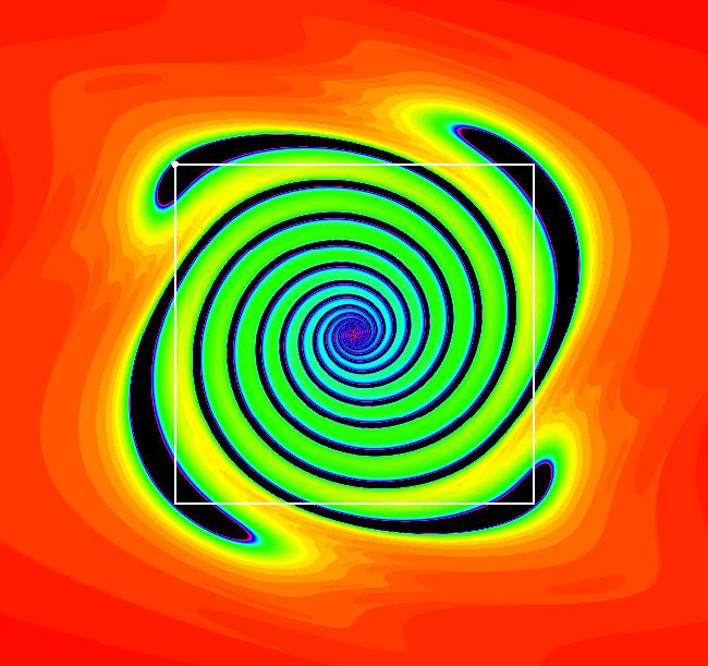
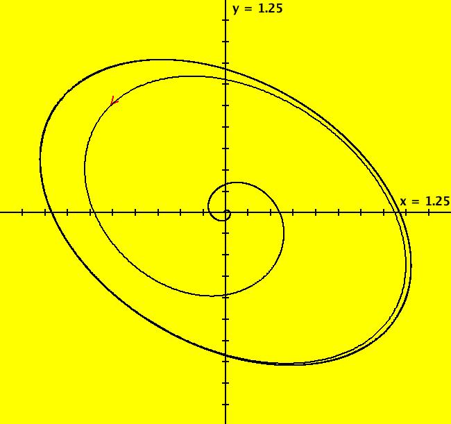
View/Sys/Gal: Ode "p. 254c, Hopf system as EMap" in "StrogatzExs." This iteration is defined by: x <- a*x-y+x*y^2, y <- x+a*y+y^3. Parameters are: a = -.4000; EMap CT: 0 Image 1: EMap view, prisoner set per-4 attractor at (-0.632560,0.631938). Image 2: Ode view, global -t limit cycle.
|
|
|
View/Sys/Gal: Ode "p. 259, fig. 8.3.3, an oscillating chemical reaction" in "StrogatzExs." This system of odes is defined by the equations: dx/dt = a-x-4*x*y/(1+x^2), dy/dt = b*x*(1-y/(1+x^2)) Parameters are: a = 10; b = 4; Adjust the control parameters to see what happens. Image 1: b = 4, fxpt at (2,5). Image 2: b = 2, limit cycle.
|
|
|
View/Sys/Gal: EMap "p. 259b, fig. 8.3.3, an oscillating chemical reaction, EMapCT5" in "StrogatzExs." This iteration is defined by: x <- a-x-4*x*y/(1+x^2), y <- b*x*(1-y/(1+x^2)). Parameters are: a = 6.000; b = 7.500; Image 1: This an EMap view of the previous system. Zoom out to see the fractal structure.
|
|
|
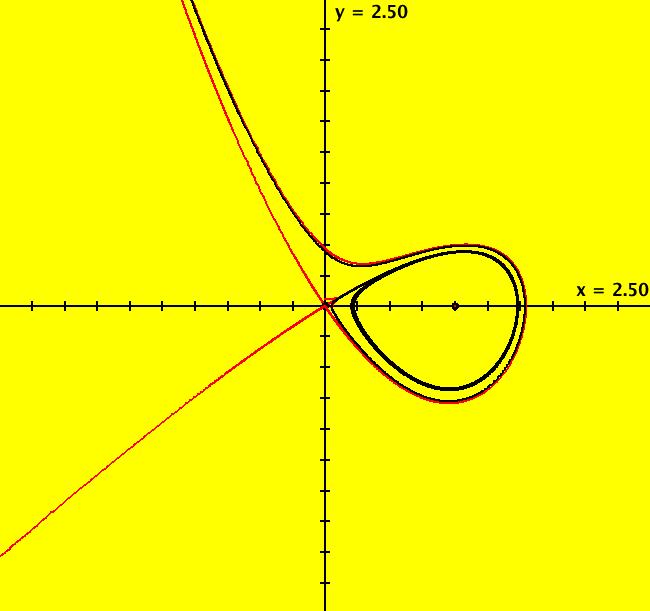
View/Sys/Gal: Ode "p. 263, fig. 8.4.3, homoclinic bifurcation" in "StrogatzExs." This system of odes is defined by the equations: dx/dt = y, dy/dt = b*y+x*(1-x+y) in the (t,x,y) coordinate system. The 1st order 2D system corresponds to the 2nd order ode: y'' = b*y'+y*(1-y+y') in the (x,y,y') coordinate system. Parameters are: b=-.9 The fixed points, at (0,0) and (1,0), are independent of b. The separatrix system, generated from ICs (0,+-.001), is shown in red. The black orbit has ICs (.099005,058845). In it either goes to (1.0), to a limit cycle (for b ~ -.87) or to infinity. In the R2+ view: Image 1: b = -1, orbit goes to (1,0). Image 2: b = -.87, orbit goes to a limit cycle. Image 3: b = -.86, orbit goes to infinity. For more details see: homoclinic bifurcation.
|
|
|
View/Sys/Gal: Ode "p. 318 & 319, figs. 9.3.1 & 9.3.2, 3D Lorenz attractor" in "StrogatzExs." This system of odes is defined by the equations: dx/dt = s*(y-x), dy/dt = r*x-y-x*z, dz/dt = x*y-b*z Parameters are: s=10; r=28; b=2.6667 ICs are t = 0, x = y = z = .2 In all views, the solutions have been extended to t = 100. Image 1: The (x,z) view. Click the "Center" button to watch the image being drawn. In the (t,*) views, make the viewing area wider by setting hMax to 100. Image 2: The (t,x,z) view with hMax = 100. In the (x,z) view, to see the attractor "attract," click the Clear button then click the Flow button and start 20 random dots. To see an animation of the motion, Clear the view and right click in the graphics area to start a solution at (t,x,y,z) = (0,5,0.2,9) in the (x,z) view. Extend the solution forward in time then click the Flow button. With no random dots, run the animation for about 40 seconds. In the (t,x) view, there are actually two different solutions defined, the first uses ICs: t = 0, x = y = z = .2 and the second uses ICs t = 0, x = y = z = .20000001 Watch as the two curves are being drawn and note that they begin to differ at about t = 30. This shows that the system is very sensitive to the ICs. To edit the (t,*) curves, click on the arrowhead. You may need to pan left to click on the arrowhead but once you open the curve controller you can pan right to un-pan left.
|
|
|
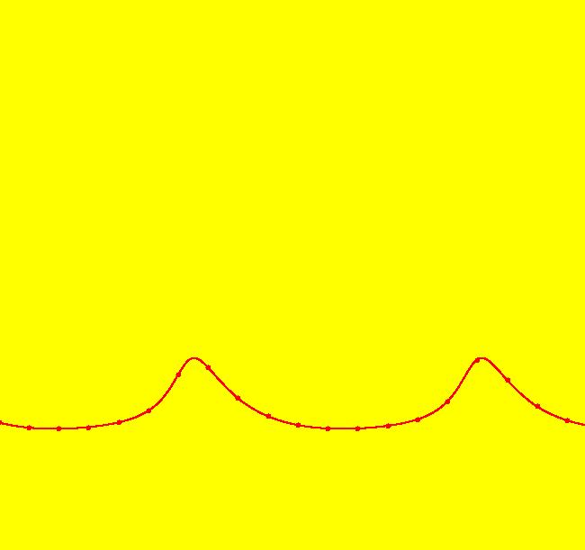
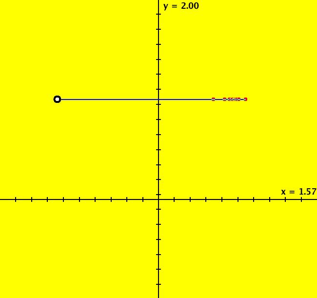
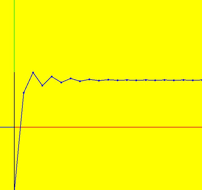
View/Sys/Gal: IMap "p. 352, fig. 10.1.6, 1D IMap1000 as x <- cos(x), y <- 1" in "StrogatzExs." This IMap system is defined by: x <- cos(x), y <- 1 converges to the limit point (x,y) = (0.7390851332151607,1). ICs are (t,x,y) = (0,-1,1). Image 1: The motion is on the blue line. To animate the motion click the Flow button. Image 2: You can also see the convergence to the limit point by setting hMax = 20 and going to the 3D/(t,x) view. To see the coordinates at the limit point to full machine precision select "Show Last +t Point" on the Settings menu. You should get: last (x,y,t) = (0.7390851332151607, 1.0, 10024.0)
|
|
|
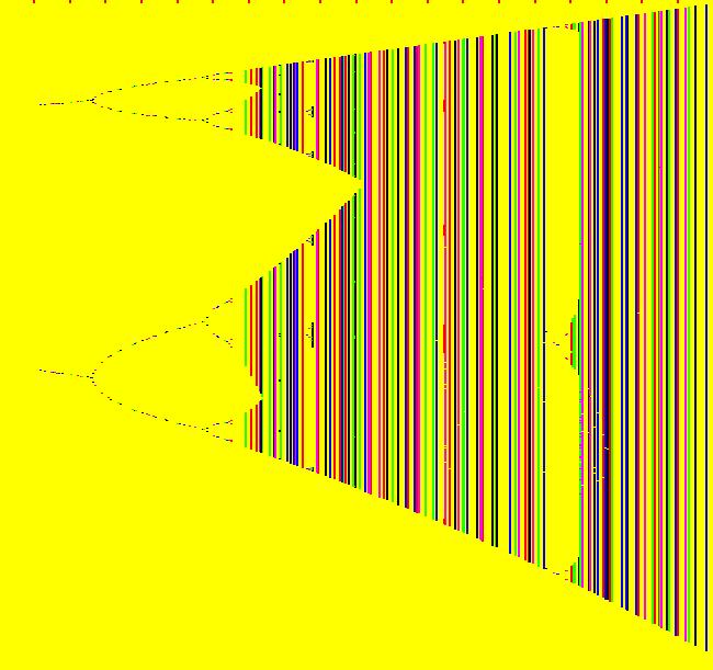
View/Sys/Gal: IMap "p. 357, fig. 10.2.7, bifurcation diagram for logistic IMap0001" in "StrogatzExs." This 2D IMap system: x <- x, (B) y <- x*y*(1-y) is the bifurcation diagram for the 1D logistic map: x <- r*x*(1-x), (A) for x ∈ [0,1], r ∈ [0,4] In (B), "x" plays the role of parameter r in (A) and "y <- x*y*(1-y)" plays the role of the logistic map. A large number orbits have been started near the bottom of the graphics area. You may need to wait for the orbits to be drawn. Image 1: Bifurcation diagram for x <- r*x*(1-x). Find "r" values for system (A) orbits of periods: 2, 4 and 8. To do this, select "Show Approximate IMap Orbit Period" on the Help menu then start an orbit near x = 3.418 then near x = 3.504 then near x = 3.551. If you select Flow after you start each orbit you can watch the convergence to the periodic orbit.
|
|
|
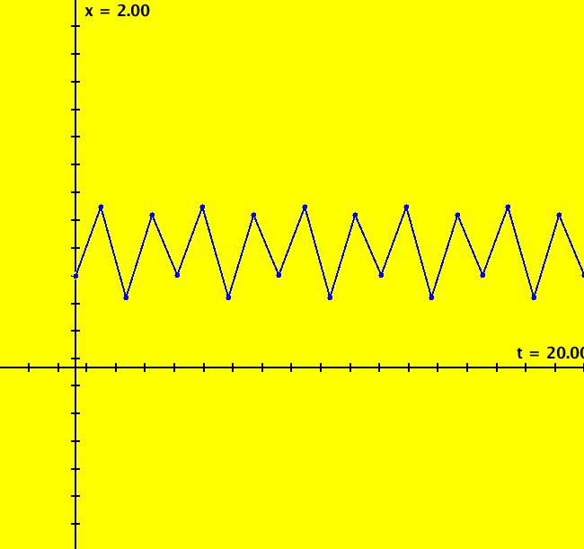
View/Sys/Gal: IMap "p. 357b logistic equation IMap1100" in "StrogatzExs." This iteration is defined by: x <- r*x*(1-x). Parameters are: r=3.5 Image 1: In the IMap view, seed at (0,.5) gives a period-4 cycle. Go to the Ode view and turn S On. Image 2: In the Ode view, IC at (0,.5) gives a trajectory that goes to x(-infinity) = 0 and x(+infinity) = 1.
|
|
|
View/Sys/Gal: Ode "p. 377, fig. 10.6.6, 3D Rossler system" in "StrogatzExs." This is the 3D Rossler system. The system of odes is defined by the equations: dx/dt = -y-z, dy/dt = x+a*y, dz/dt = b+z*(x-c) Parameters are: a = .20; b = .20; c = 2.40; p(0) = (4.424,0,1.54) is close to a limit cycle with period 34.452. Image 1: The 2D (x,y) view. In this view the unlabeled +z-axis is perpendicular to the screen toward the viewer. To get to the 3D (x,y,z) view, select z as well as x and y. Image 2: The 3D/(x,y,z) view with (yaw,pitch,roll) = (30,15,0). The (x,y,z) axes are (red,green,black). The +t part of the trajectory is red. Image 3: 3D/(x,y,z) view with yaw = 0, c = 4.
|
|
|
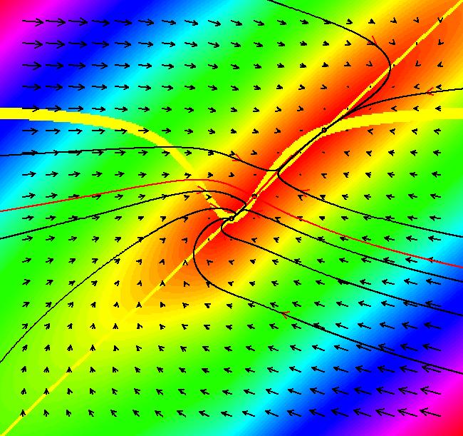
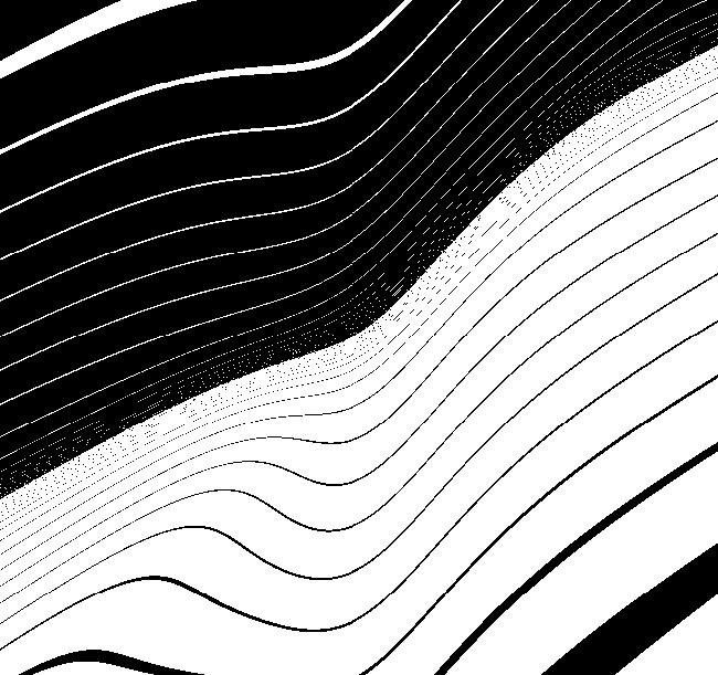
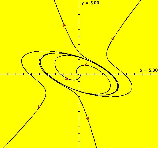
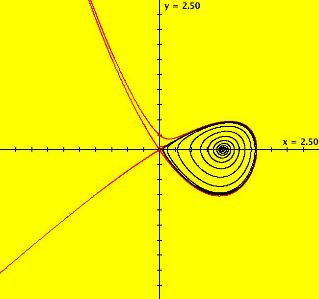
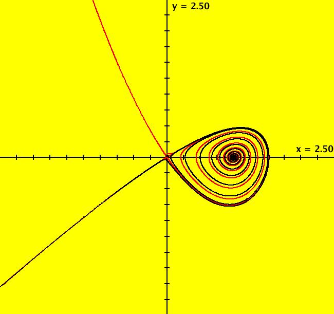
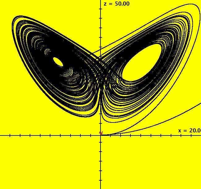
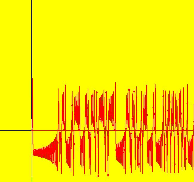
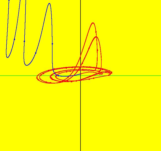
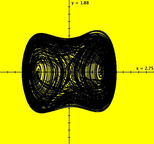
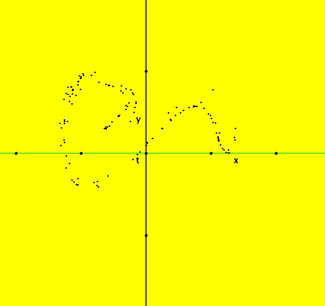
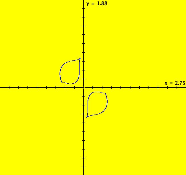
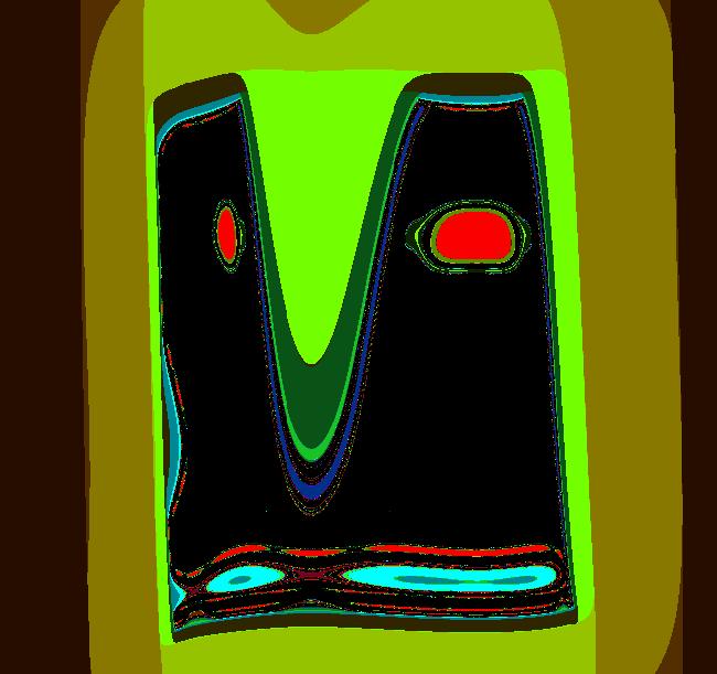
View/Sys/Gal: Ode "p. 446, fig. 12.5.6, Poincare map" in "StrogatzExs." See Strogatz p. 443, Guckenheimer and Holmes, p. 82 and Takashi Kanamaru. Note that the system contains "t" so it is non-autonomous. This system is called a "forced double-well oscillator." It is a form of the Duffing equation. The system of odes is defined by the equations: dx/dt = y, dy/dt = -.25*y+x-x^3+f*cos(t) Parameters are: f = .40; Image 1: The Ode view in the (x,y) plane. The solution starts at (t,x,y) = (0,0,0) and extends past t = 2000 to generate the Poincare Map, PMap for short. The PMap is a t-strobed view of a continuous trajectory while the IMap is the orbit of a discrete iteration. The PMap shows points (x(t),y(t)) on an Ode trajectory, computed by RK4 in continuous time, at t = n*2* π where n is an integer. Image 2: The PMap Ode 3D/(x,y) view indicates a chaotic trajectory. The IMap shows points (x(t),y(t)) on the orbit of the discrete-time iteration: x <- y, y <- -.25*y+x-x^3+f*cos(t) where t is an integer >= 0. Image 3: The IMap view shows a two part chaotic attractor. Image 4: The EMap CT2 view, with f = -1.1, gives another "art" image. One final thing to try - in the Ode view, clear the trajectory then start a new trajectory at (0,0). Extend it in +t and start a flow animation (no dots, speed = max, duration = 40 sec) to see the chaotic motion.
|

