Click on an image to go directly to a system or scroll to see the systems in this gallery.
 |
 |
 |
 |
 |
 |
 |
 |
 |
 |
 |
 |
 |
 |
 |
 |
 |
 |
 |
 |
 |
 |
 |
 |
 |
 |
 |
 |
 |
 |
 |
 |
 |
 |
 |
 |
 |
 |
 |
 |
 |
 |
 |
 |
 |
 |
 |
 |
 |
 |
 |
 |
 |
 |
 |
 |
 |
 |
 |
 |
 |
 |
 |
 |
 |
 |
 |
 |
 |
 |
 |
 |
 |
 |
 |
 |
 |
 |
 |
 |
 |
 |
 |
 |
 |
 |
 |
 |
 |
 |
 |
 |
 |
 |
 |
 |
 |
 |
 |
 |
 |
 |
 |
 |
 |
 |
 |
 |
 |
 |
 |
 |
 |
 |
 |
 |
 |
| OdeFactory Images and Annotations | |||||||||||||||||||||||||||||||||||||||||||||||||||||||||||||||||||||||||||||||||||||||||||||||||||||||||||||||||||||||||||||||||||
|
An OdeFactory Slide Show Click on a slide to zoom in. Click "video" to see a video. |
Sys: Introduction to Finding IMap Cycles Introduction to Finding IMap Cycles (1) The 2D linear vector field: (y,-a*x), with a = 1, generates only cycles in both the Ode and IMap views. The cycles are circles of period 2 π in the Ode view and the corners of squares of period 4 in the IMap view. For a ≠ 1, the trajectories in the Ode view and the orbits in the IMap view are spirals. (2) Systems (2a) through (2s) explore properties of the well studied logistic map: x <- r*x*(1-x). Systems (2f) demonstrate finding the Feigenbaum constants for the logistic map. System (2m), based on he article by Robert M. May, (1979) contains a nice discussion of the complex dynamics of the logistic map. Systems (2s) are logistic map examples from the textbook "Nonlinear Dynamics and Chaos" by Strogatz, p. 353-366. Also, copy/paste logistic map or logistic map r=3.569935 into WA to find out more about the logistic map. (3) The 2D nonlinear vector fields: (a) (y-sin(x),a-x), (b) (y-cos(x),a-x) and (c) (y-sgn(x)*sqrt(abs(b*x-c)),a-x) produce interesting images in the IMap view which contain many complicated periodic orbits. In particular, see the "(3d) IMap0111 KAM islands ..." example. For further details, see the article by Barry Martin, "Graphic Potential of Recursive Functions" in "Computers in Art, Design and Animation," 1989, pages 109-129. (4) System (4) is an example of a simple system for which the mathematical and the computational properties are completely different. Consider the 1D left shift map: x <- 10*x%1. Call an orbit of the 1D system which starts at a rational point x(0) a rational orbit. Mathematically: (a) All rational orbits are periodic and all irrational orbits are not periodic. (b) The system is totally chaotic in that for any rational orbit P(x(0)) no nearby orbit stays close to P(x(0)). Computationally: (a) Every orbit goes to the fixed point x = 0. (b) The system is not chaotic. If 1D system (A) is x <- r*f(x) then 2D system (B) x <- x, y <- x*f(y), gives the bifurcation diagram of system (A). (5) Systems (5) concern the 1D tent map and the corresponding 2D bifurcation map. (6) Systems (6) concern the 2D2P Lozi system, defined by the vector field: L(a,b) = (1-a*abs(x)+b*y,x) which has many interesting properties. A dozen examples illustrate various features of the Lozi system in the: EMap, IMap and Ode views. See Lozi maps or the 2013 book by Zeraoulia Elhadj on Lozi maps at Amazon.com. Quoting from the Amazon page: "This book is a comprehensive collection of known results about the Lozi map, a piecewise-affine version of the Henon map. The Henon map is one of the most studied examples in dynamical systems and it attracts a lot of attention from researchers, however it is difficult to analyze analytically. Simpler structure of the Lozi map makes it more suitable for such analysis. The book is not only a good introduction to the Lozi map and its generalizations, it also summarizes of important concepts in dynamical systems theory such as hyperbolicity, SRB measures, attractor types, and more." (7) Systems (7) are "Standard" map examples. (8) Systems (8) are variations of the 1D quadratic map.
|
||||||||||||||||||||||||||||||||||||||||||||||||||||||||||||||||||||||||||||||||||||||||||||||||||||||||||||||||||||||||||||||||||
|
|
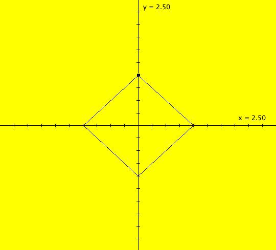
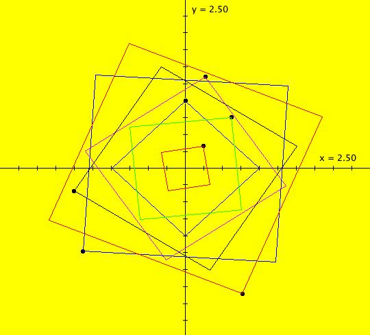
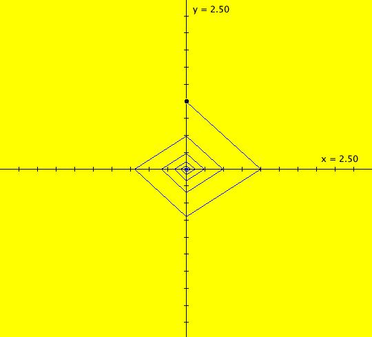
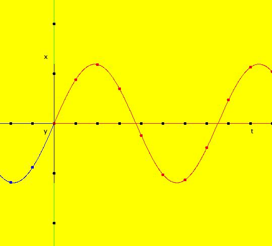
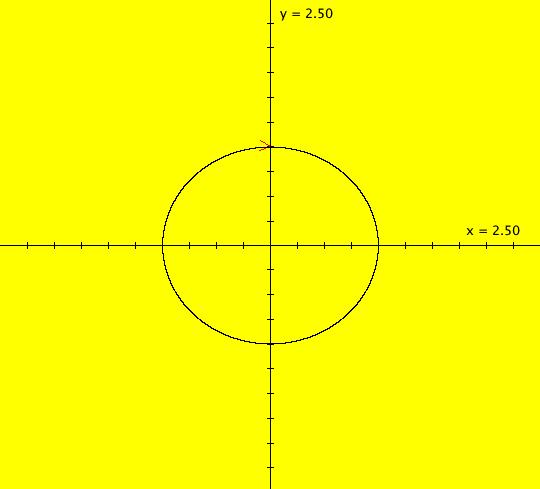
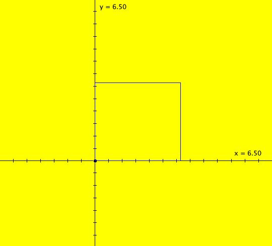
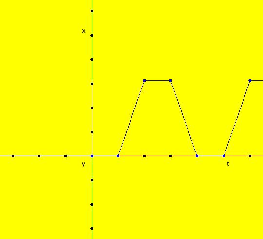
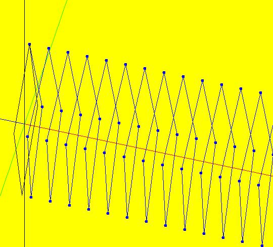
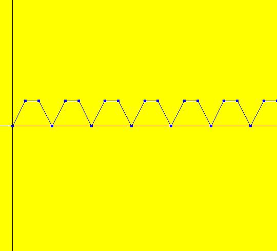
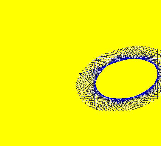
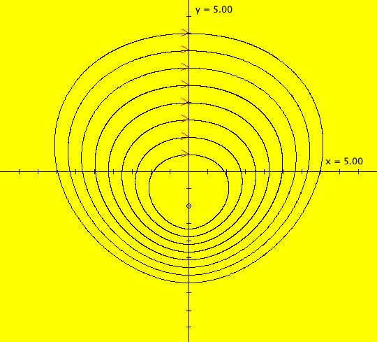
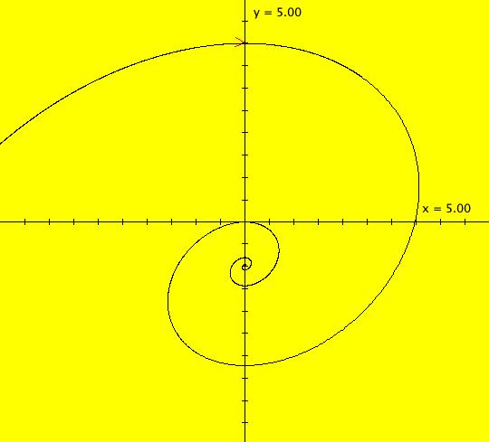
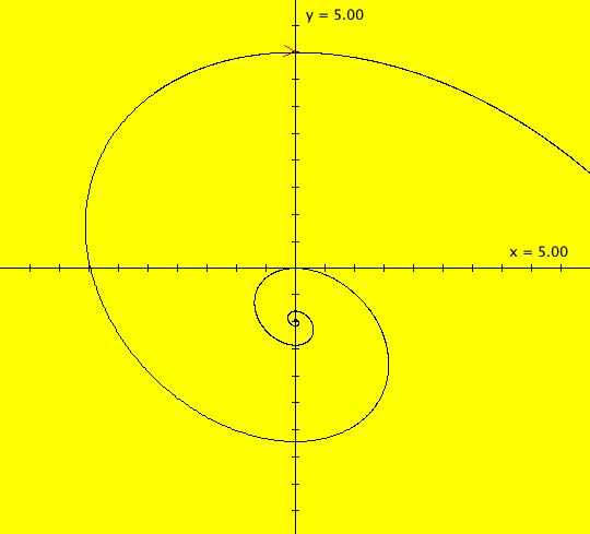
Sys: (1) IMap1100, (y,-a*x), a=1, cycle w/per 4 This iteration is defined by: x <- y, y <- -a*x. Parameters are: a=1 For a = 1, every orbit is periodic with period-4. This is easy to see. With a = 1, for any seed value (x,y), the iteration is x <- y, y <- -x or, as a list, (x,y) goes to (y,-x). In words: "at each step, the 1st item in the list is replaced by the 2nd item and the 2nd item is replaced by the negative of the former 1st item" so So - (x,y) goes to (y,-x) which goes to (-x,-y) which goes to (-y,x) which goes to (x,y). Note that OdeFactory will report a period-4 orbit for the system x <- y, y <- -.99999*x. This is because the algorithm used looks for a close first-return, not an exact first-return. So - when trying to find periodic orbits in 2D IMaps, always turn "Show 2D IMap Orbit Sequence" on to see if the orbit "looks" periodic. When the system is selected, the flag values "1100" appended to "IMap" in the system's name turn on "Show 2D IMap Orbit Sequence" and "Show Approximate Period," on the Settings menu. Image 1: IMap with a single seed at (0,1). Try various seeds (ICs). Click "Center" to update orbit colors as you add seeds. Image 2: Several period-4 IMap orbits. If a > 1 all IMap orbits spiral in and if a < 1, all orbits spiral out. Image 3: IMap with a = .7 case, spiral in. Image 4: Ode 3D/(t,x) view w/ICs (0,1), a = .7, period = 7.510. Image 5: Ode view w/ICs (0,1), a = 1, period = 2*pi.
|
||||||||||||||||||||||||||||||||||||||||||||||||||||||||||||||||||||||||||||||||||||||||||||||||||||||||||||||||||||||||||||||||||
|
|
Sys: (2a) 1D IMap1100, x <- (3.5+b*.1)*x*(1-x), logistic map Generally the logistic map is written as: x <- r*x*(1-x), where r is the bifurcation parameter. I want to look at values of r near 3.5 so I rewrote r as (3.5+b*.1). This iteration is defined by: x <- (3.5+b*.1)*x*(1-x). Parameters are: b = -1.00; A trajectory/orbit has been started at (0,0.5). Image 1: A period 2 cycle, b = -1. The red dots show the beginning and end of the cycle. In the IMap view slowly increase b and watch what happens. Image 2: A period 8 cycle, b = .5. To observe chaotic behavior due to slightly different starting values, start a second orbit at (0,.500001) then set b = 2.5. Image 3: Seeds (0,.5) and (0,.500001) with b = 2.5 Image 4: Seeds (0,.5) and (0,.500001) with b = 2.4, a 5-cycle. Reference: logistic map.
|
||||||||||||||||||||||||||||||||||||||||||||||||||||||||||||||||||||||||||||||||||||||||||||||||||||||||||||||||||||||||||||||||||
|
|
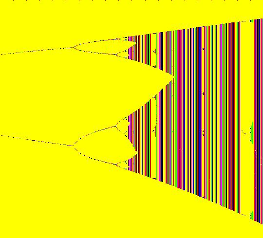
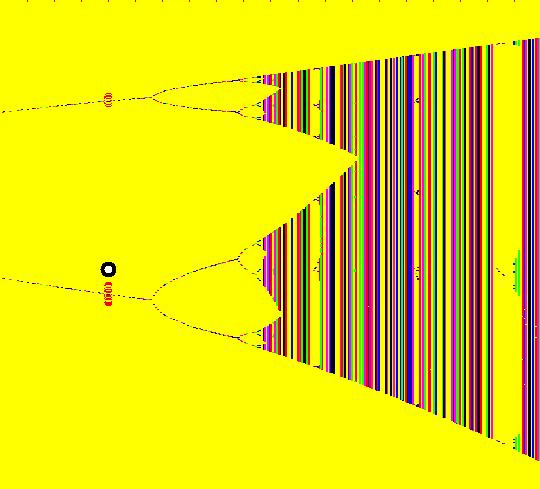
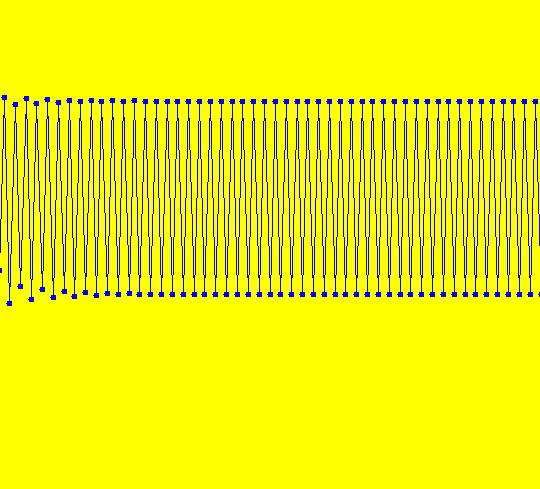
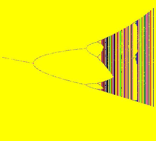
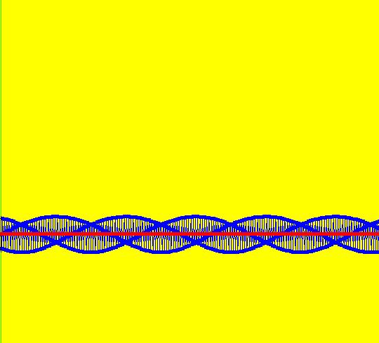
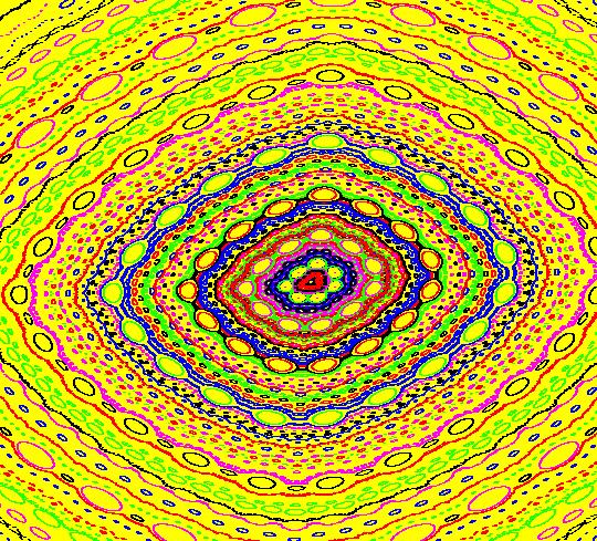
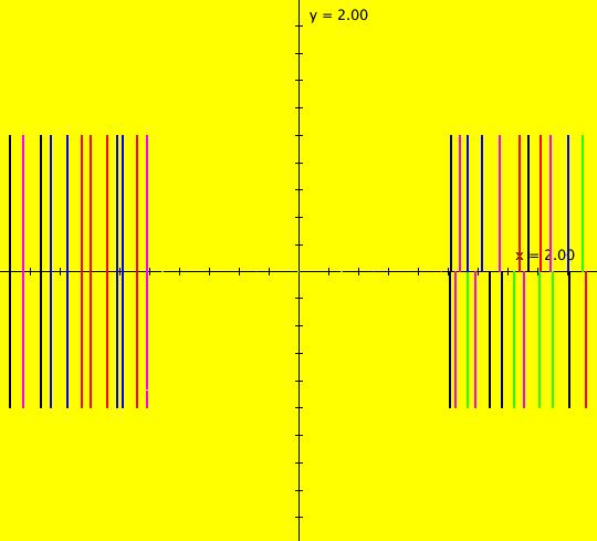
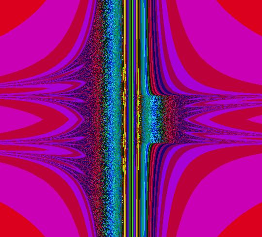
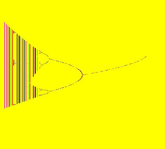
Sys: (2b) 2D IMap0101, x <- x, y <- x*y*(y-1), logistic bifurcation map This is the bifurcation diagram of the 1D logistic map x <- b*x*(1-x), where b is the bifurcation parameter. The image is also called a Feigenbaum diagram. Image 1: Bifurcation diagram for the logistic map. As we shall see, in OdeFactory, it is really just another 2D IMap. The diagram is generated by first replacing x by y and then rewriting the 1D iteration as y <- b*y*(1-y). Next replace the bifurcation parameter b by the variable x and consider the 2D system: x <- x, (x now plays the role of b) y <- x*y*(1-y) (the original 1D map) The IMap view of the 2D system shows 322 orbits of the 1D system as dots projected onto the vertical lines x = b. The open regions delineated by the horizontal dotted lines from approximately x = 3.28 to x = 3.44 to x = 3.54 to x = 3.563 are called "windows." Orbits starting in the 1st window have period 2, those starting in the second window have period 4, those starting in the 3rd window have period 8 etc. Starting on the left, the open "windows" in the bifurcation show the period-doubling of the periodic orbits. Click in the windows to start a new and see its period. See "Nonlinear Dynamics and Chaos," by Steven Strogatz p. 357 fig 10.2.7 for more details. To generate the bifurcation diagram, start several orbits in the IMap view. Vertical lines with n dots are period-n orbits of the 1D system. Solid vertical lines are chaotic orbits of the 1D system. To view an orbit of period 2, start an orbit at (3.4,.5) and run a Flow animation. You will see red dots accumulating on the line x = 3.4 at about y1 = .447 and y2 = .839. The extra red dots near y1 and y2 are due to the transient part of the orbit starting at t = 0. The periodic orbit is really a limit orbit or limit cycle. Image 2: After a Flow animation of the limit orbit at (3.4,.5). Another way to view this orbit is to clear the view, start the orbit again, change hMax to 100 and go to the 3D/(t,y) view to see the time-series for the orbit. Image 3: A single orbit at (3.4,.5) in the 3D/(t,y) view with 0 <= t <= 100. If you go back to system (2a) 1D IMap1100, ((3.5+b*.1)*x*(1-x)), b = -1.00; you will see that the min and max on the x(t) curve are at about x = .447 and x = .839. The extra dots on the x = 3.4 line when you run the Flow animation in the 2D IMap view are the first few iteration points. You don't see them in the 1D example since the t axis is from 2495 to 2510, i.e. the transient part of the iteration is not shown. Problem 1: find a period-3 orbit and display it in the 1D system. Solution: the large window on the right looks like it corresponds to a 3-cycle. Click in the window to check this out. Clicking at about (x,y) = (3.831111,0.593939) gives a 3-cycle. Now go to the 1D system and select b such that (3.5+b*.1) = 3.831111, that is, b ~ 3.3 Problem 2: show that the 2D IMap image is a fractal. Solution: select a small window, say the lower 8-cycle window, then zoom in on it. Image 4: Selecting a small 8-cycle window. Clear the orbits and create new orbits to regenerate the smaller IMap. Do it again with a 16-cycle window, then with a 32-cycle window. Image 5: Lower 8-cycle window zoomed in with orbits added.
|
||||||||||||||||||||||||||||||||||||||||||||||||||||||||||||||||||||||||||||||||||||||||||||||||||||||||||||||||||||||||||||||||||
|
|
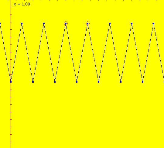
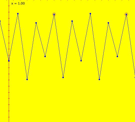
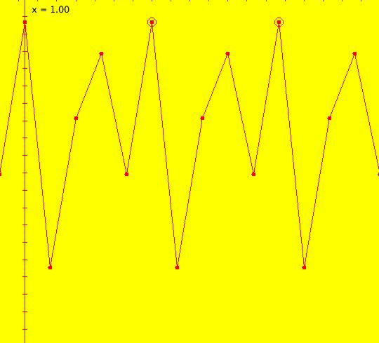
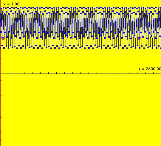
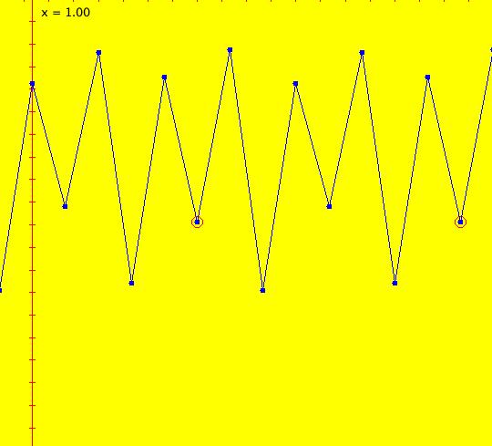
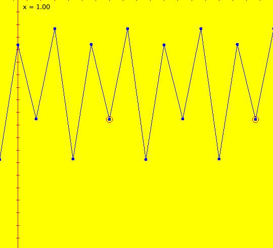
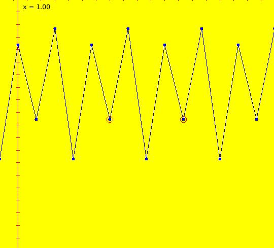
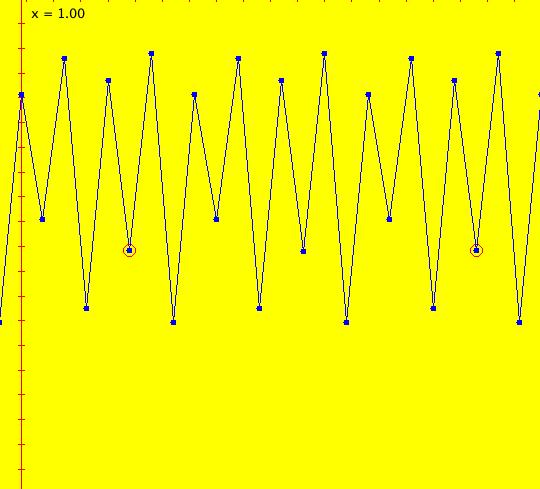
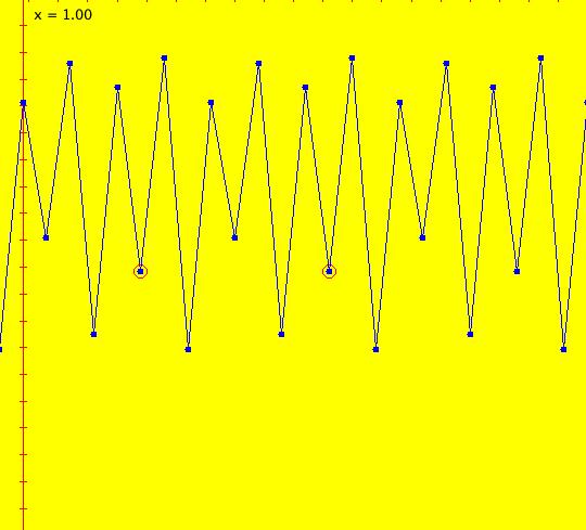
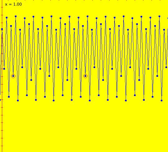
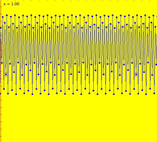
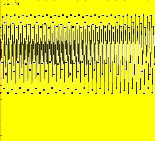
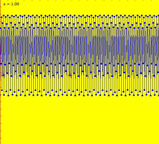
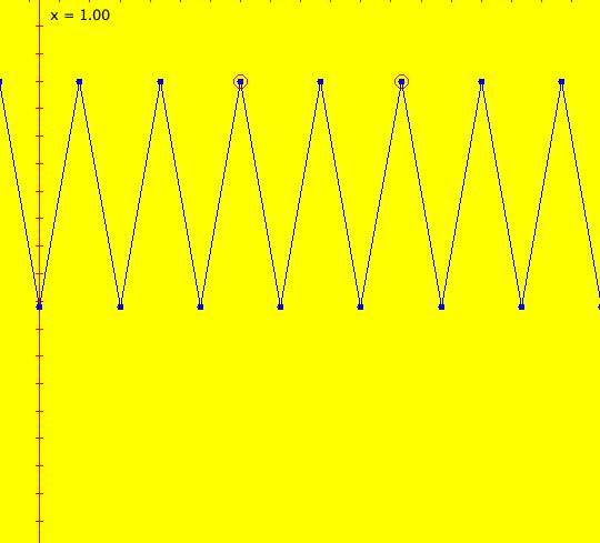
Sys: (2c) WA, IMap0100, (r*x*(1-x)), r=3.56994 This iteration is defined by: x <- r*x*(1-x). Parameters are: r=3.56994 ICs: (t,x) = (0,0.1). In OdeFactory, the approximate period of a 1D IMap orbit, or limit cycle, is the first time for which the condition abs(x(t)-x(startingStep)) < perEps is satisfied where startingStep = 2500 and perEps = .000004. The large value of startingStep is used to get past the transient part of the orbit. Image 1: IMap view with a period-256 cycle. Look for the two red circles, three rows of blue dots up from the bottom. The red circles mark the start and end of one period of the period-256 cycle. Near values of r where the period changes, or where the orbits become chaotic, the approximate period becomes very difficult to compute. Copy/paste logistic map r = 3.56994 into WA to see what you get.
|
||||||||||||||||||||||||||||||||||||||||||||||||||||||||||||||||||||||||||||||||||||||||||||||||||||||||||||||||||||||||||||||||||
|
|
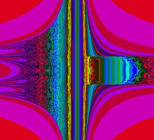
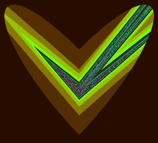
Sys: (2d) 2D EMapCT6 ((1+s*.1)*x,(1+s*.1)*x*y*(1-y)), s = .700; This iteration is defined by: x <- (1+s*.1)*x, y <- (1+s*.1)*x*y*(1-y). Parameters are: s = .700; This is a time-scaled version of the logistic bifurcation diagram, system (2b), in a different region of the plane, in the EMap view. Image 1: EMap of time-scaled logistic map bifurcation diagram w/CT 6.
|
||||||||||||||||||||||||||||||||||||||||||||||||||||||||||||||||||||||||||||||||||||||||||||||||||||||||||||||||||||||||||||||||||
|
|
Sys: (2f) IMap0100 2<->4 (R*x*(1-x)), b=0, R=3.4494897+b The (2f) series of systems illustrates period-doubling in the logistic map.
Reference: Feigenbaum constants. The R values in the table indicate the right edges of the first few period windows. Good values for R can be difficult to compute, particularly as the periods increase. Decreasing R, by decreasing b, decreases the period by a factor of 2. The logistic map is defined by: x <- R*x*(1-x). Parameters are: b=0 Functions are: R=3.4494897+b Image 1: A 4-cycle. Decrease b to get a 2-cycle. Image 2: b = -.002 gives a 2-cycle. Increase b to get an 8-cycle. Image 3: b = .1 gives an 8-cycle.
|
|
Sys: (2f) IMap0100 4<->8 (R*x*(1-x)), b=0, R=3.5440903+b This iteration is defined by: x <- R*x*(1-x). Parameters are: b=0 Functions are: R=3.5440903+b Here we are just on the 8-cycle side of the 4-cycle to 8-cycle boundary. Image 1: b = 0, gives an 8-cycle. Decrease b to get a 4-cycle. Image 2: b = -.001, gives a 4-cycle.
|
|
Sys: (2f) IMap0100 8<->16 (R*x*(1-x)), b=0, R=3.5644073+b This iteration is defined by: x <- R*x*(1-x). Parameters are: b=0 Functions are: R=3.5644073+b This is the "16" edge of the 8 to 16 cycle boundary. Image 1: b = 0, 16-cycle. Decrease b to get an 8-cycle. Image 2: b = -.001, 8-cycle.
|
|
Sys: (2f) IMap0100 16<->32 (R*x*(1-x)), b = 0; , R=3.5687594+b This iteration is defined by: x <- R*x*(1-x). Parameters are: b = .000; Functions are: R=3.5687594+b Image 1: b = 0, 32 cycle. Decrease b to get a 16-cycle. Image 2: b = -.001, 16 cycle.
|
|
Sys: (2f) IMap0100 32<->64> (R*x*(1-x)), b=0, R=3.5696916+b This iteration is defined by: x <- R*x*(1-x). Parameters are: b=0 Functions are: R=3.5696916+b Image 1: b = 0, 64 cycle. Decrease b to get a 32-cycle. Image 2: b = -.001, 32 cycle.
|
|
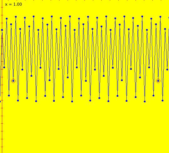
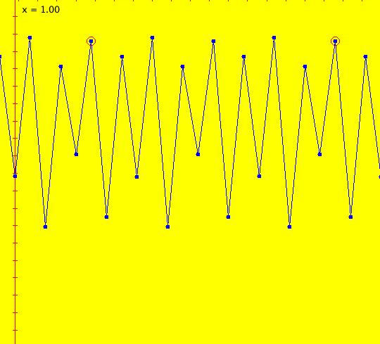
Sys: (2f) IMap0100 64<->128 (R*x*(1-x)), b=0, R=3.5698913+b*.01 This iteration is defined by: x <- R*x*(1-x). Parameters are: b=0 Functions are: R=3.5698913+b*.01 Image 1: b = 0, 128 cycle. Decrease b to get a 64-cycle. Image 2: b = -.001, 64 cycle.
|
|
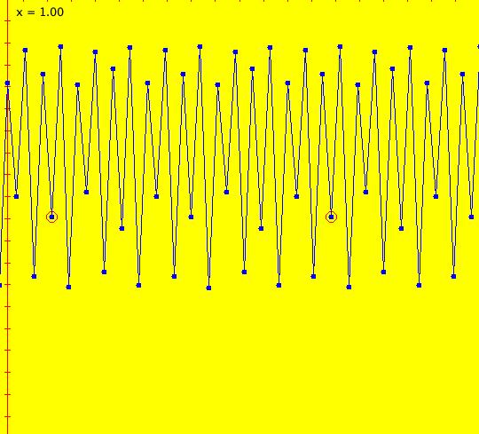
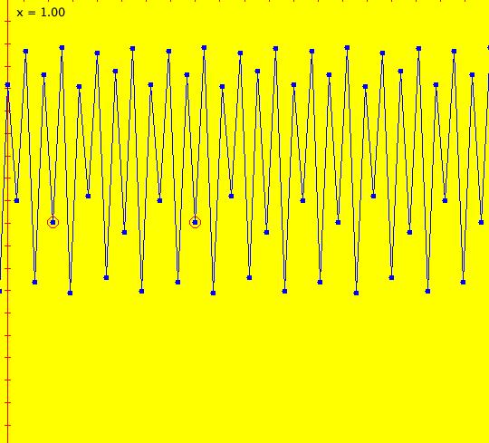
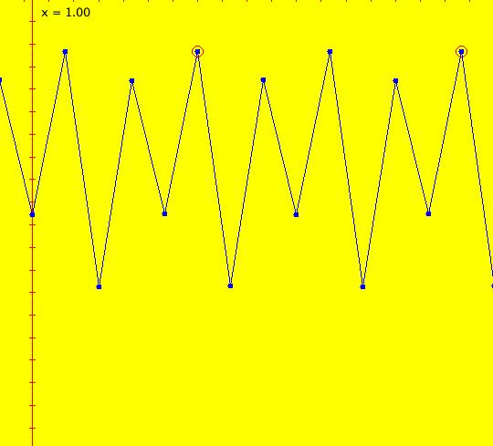
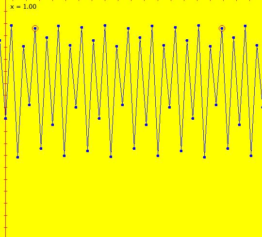
Sys: (2f) IMap0100 128<->256 (R*x*(1-x)), b=0, R=3.5699340+b*.01 This iteration is defined by: x <- R*x*(1-x). Parameters are: b=0 Functions are: R=3.5699340+b*.01 Image 1: b = 0, 256 cycle. Decrease b to get a 128-cycle. Image 2: b = -.001, 128 cycle.
|
|
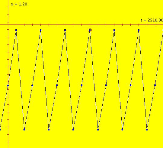
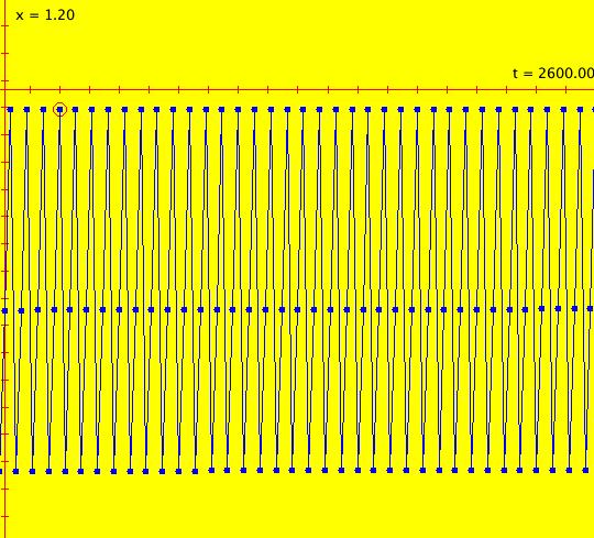
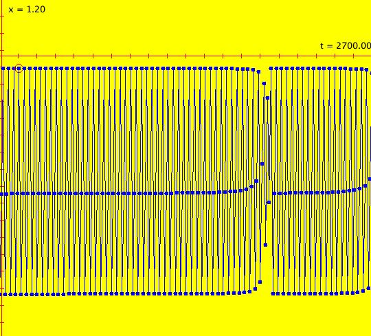
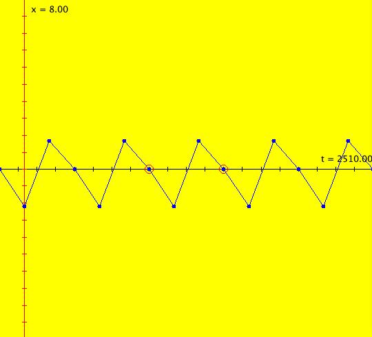
Sys: (2m) p. 462, R. M. May, IMap0100, (r*x*(1-x)), r=3.8284, cycle w/per 3 This iteration is defined by: x <- r*x*(1-x). Parameters are: r = 3.8284 See the table at the bottom of page 462 of the 1979 paper by R. M. May. R. M. May, and WA, report a 3-cycle, OdeFactory reports a 890-cycle. The orbit is most likely chaotic. To see this, set increase hMax. Image 1: hMax = 2510, looks like a 3-cycle. Image 2: hMax = 2600, still looks like a 3-cycle. Image 3: hMax = 2700, now it looks chaotic.
|
|
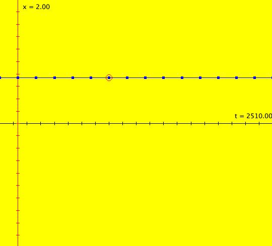
Sys: (2s) p. 352, fig. 10.1.3, IMap0100 (cos(x)) The page numbers in systems (2s) refer to pages in the textbook "Nonlinear Dynamics and Chaos," by Strogatz. This iteration is defined by: x <- cos(x). ICs: (t,x) = (0,-1) All orbits go to the fixed point, x = 0.739... which is the solution to x = cos(x). Apply WA to x = cos(x) to find x to more places. Check WA against OdeFactory. Image 1: The "period-1 cycle" i.e. fixed point at x = 0.7390851332151607...
|
|
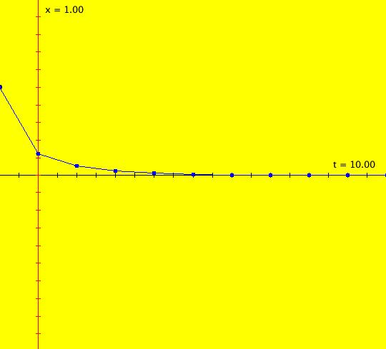
Sys: (2s) p. 353, IMap0100 (r*x*(1-x)), r=.5, x -> 0 for 0 <= r < 1 This iteration is defined by: x <- r*x*(1-x). Parameters are: r=.5 The interesting range for the control parameter is 0 <= r <= 4. For 0 <= r < 1, x -> 0. For 1 < r < 3, x -> a steady state, i.e. a fixed point. ICs: (t,x) = (0,1) The fixed point is at x = 6.112663368688884E-62 ≈ 0. Image 1: 2495 <= t <= 2510 shows the steady state. Image 2: 0 <= t <= 10 shows the transient.
|
|
Sys: (2s) p. 354, fig. 10.2.2, IMap0100 (r*x*(1-x)), r=2.8, x -> a steady state This iteration is defined by: x <- r*x*(1-x). Parameters are: r=2.8 ICS: (0,.5) Fixed point: x = 0.6428571428571428 Apply WA to x = 2.8*x*(1-x) to get x = 0.642857 Image 1: r = 2.8 Vary r and watch the fixed point change. Note: In the IMap view the fixed point condition is; x <- x, i.e. x = r*x*(1-x). In the Ode view, the fixed point condition is: dx/dt = 0, i.e. 0 = r*x*(1-x). So the Ode fixed points are at x = 0 and x = 1 independent of r.
|
|
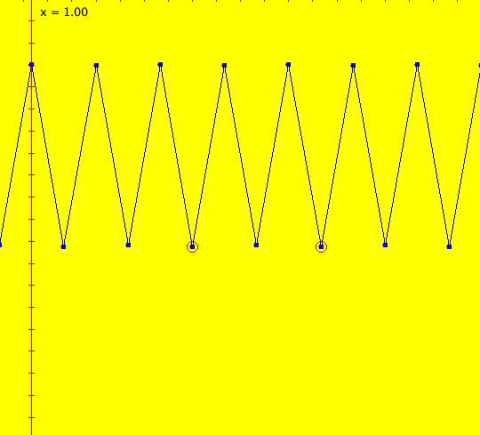
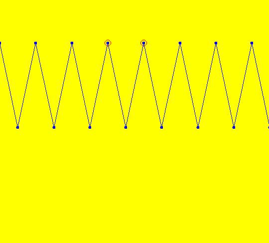
Sys: (2s) p. 354, fig. 10.2.3, IMap0110, (r*x*(1-x)), r=3.3, cycle w/per 2 This iteration is defined by: x <- r*x*(1-x). Parameters are: r=3.3 ICS: (t,x) = (0,.5) The first point circled is the starting point and the second point circled is the approximate first-return point. Image 1: A period-2 orbit.
|
|
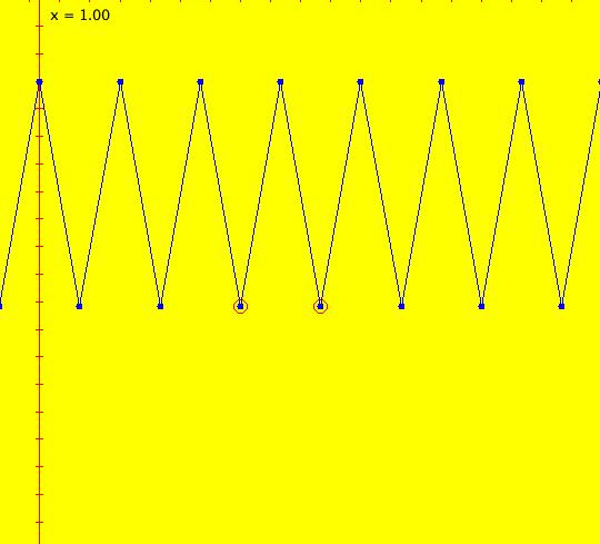
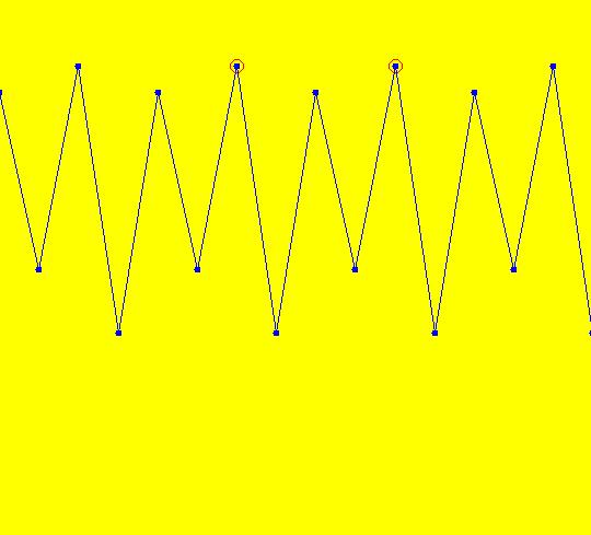
Sys: (2s) p. 354, fig. 10.2.4, IMap0110 (r*x*(1-x)), r = 3.5, cycle w/per 4 This iteration is defined by: x <- r*x*(1-x). Parameters are: r = 3.5 ICS: (t,x) = (0,.5) Image 1: A 4-cycle.
|
|
Sys: (2s) p. 355, IMap0100, (r*x*(1-x)), r=3.449, cycle w/per 4 This iteration is defined by: x <- r*x*(1-x). Parameters are: r=3.449 Image 1: OdeFactory and Strogatz give a 4-cycle while WA gives a 2-cycle. r = 3.4494897 is the 2-4 boundary so 2-cycle is the correct answer.
|
|
Sys: (2s) p. 355, IMap0100, (r*x*(1-x)), r=3.54409, cycle w/per 8 This iteration is defined by: x <- r*x*(1-x). Parameters are: r=3.54409 Image 1: OdeFactory and Strogatz give an 8-cycle while WA gives a 4-cycle. r = 3.5440903 is the 4-8 boundary so 4 is the correct answer.
|
|
Sys: (2s) p. 355, IMap0100, (r*x*(1-x)), r=3.5644, cycle w/per 16 This iteration is defined by: x <- r*x*(1-x). Parameters are: r=3.5644 Image 1: A 16 cycle.
|
|
Sys: (2s) p. 355, IMap0100, (r*x*(1-x)), r=3.568759, cycle w/per 32 This iteration is defined by: x <- r*x*(1-x). Parameters are: r=3.568759 Image 1: A 32-cycle.
|
|
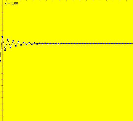
Sys: (2s) p. 355, IMap0110 ((r+b)*x*(1-x)), r = 3.569946; b = .001 This iteration is defined by: x <- (r+b)*x*(1-x). Parameters are: r = r ∞ = 3.569946; b = .001 Use b to vary r near r ∞. WA applied to logistic map r = 3.570946 says the orbit is chaotic. Image 1: The orbit looks chaotic.
|
|
Sys: (2s) p. 355, fig. 10.2.5, IMap0100 (r*x*(1-x)), r = 3.9, chaotic orbit This iteration is defined by: x <- r*x*(1-x). Parameters are: r = 3.9 OdeFactory reports a period-1635 cycle but this is actually a chaotic orbit. Image 1: A chaotic orbit.
|
|
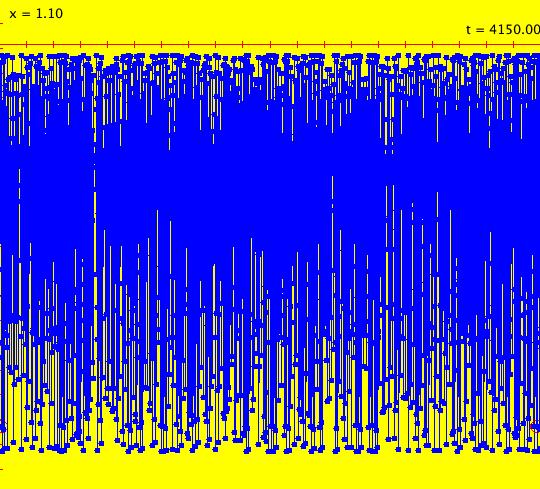
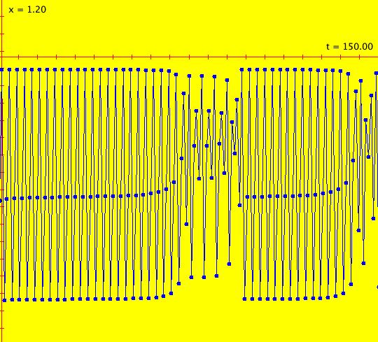
Sys: (2s) p. 363, fig. 10.4.3, IMap0100, (r*x*(1-x)), r = 3.8282, false per 3 This iteration is defined by: x <- r*x*(1-x). Parameters are: r = 3.8282 Ics: (0,.5) The system is chaotic. WA gives a false cycle of period-14. Strogatz sees the "ghost" of a 3-cycle. Image 1: t in [0,150], chaotic orbit. Image 2: t in [2495,3000].
|
|
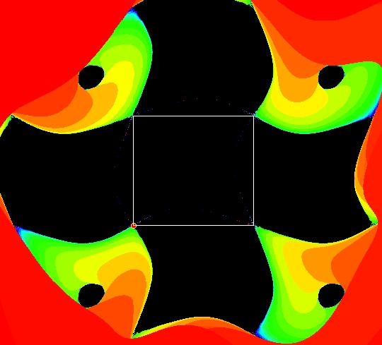
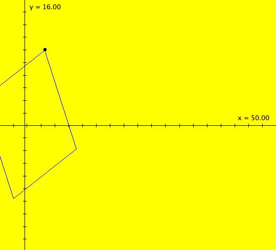
Sys: (3a) IMap1100, (y-sin(x),(pi+b*.001)-x), b=0 This iteration is defined by: x <- y-sin(x), y <- (pi+b*.001)-x. Parameters are: b=0 ICs: (x,y) = (0,0) give a 4-cycle. (0,0) -> (0,pi) -> (pi,pi) -> (pi,0) -> (0,0) Image 1: An isolated IMap 4-cycle. Image 2: The 3D/(t,x) view. Image 3: The EMap view. The 4-cycle is the white square. Image 4: The Ode view with a period 6.467 limit cycle at (x,y) = (6.090797,2.909334). From, a Barry Martin article in "Computers in Art, Design and Animation," 1989, p. 119. Vary b.
|
|
Sys: (3a) IMap1111, (y-sin(x),a-x), a = -2.30; This iteration is defined by: x <- y-sin(x), y <- a-x. Parameters are: a = -2.30; Image 1: An IMap view with all flags on. This 2D map has many 4-cycles. Find one. Hint: see system "(3d) IMap0111 KAM islands...".
|
|
Sys: (3b) IMap0011, (F,-a*G), a = -1.000; b = -2.300; , F=y-cos(x); G=b-x This iteration is defined by: x <- F, y <- -a*G. Parameters are: a = -1.000; b = -2.300; Functions are: F=y-cos(x); G=b-x Image 1: IMap view. For a nice "light-show," turn "Show 2D IMap Orbit Sequence" on.
|
|
Sys: (3b) IMap0011, (y-cos(x),a-x), a = -2.30; This iteration is defined by: x <- y-cos(x), y <- a-x. Parameters are: a = -2.30; Image 1: Chaos between KAM islands containing periodic orbits.
|
|
Sys: (3b) IMap0100, (y-cos(x),a-x), a=-2.30, cycle(?) w/per 737(?) This iteration is defined by: x <- y-cos(x), y <- a-x. Parameters are: a = -2.30; p1 = (-1.289029,-1.010975) gives a fixed point. p1 is the black dot in the center of the blue orbit. p2 = (-1.292696,-1.068548), the blue orbit, is a period-41651 orbit. Image 1: The orbits for p1 and p2. Image 2: With "Show 2D IMap Orbit Sequence" on, and zoom in 4X, we can see the edge of the periodic orbit. Other ways to view this system in order to see if we may have a cycle are to: (a) run a flow animation at max speed for 30 seconds or (b) view the system with hMax = 500 in the 3D/(t,x) view. Image 3: The 3D/(t,x) view with hMax = 500. The red line corresponds to the p1 orbit and the blue curve corresponds to the p2 orbit. In general it is difficult to find cycles or compute periods of cycles for IMaps. However, given a small ε > 0, you can compute the first time-of-return to within ε, of a starting point, which is what OdeFactory does. So - at best, we have a sort of quasi-period period(p, ε). In OdeFactory, p = seed + 2500 steps, ε = perEps = 0.000004 Adding 2500 iteration steps to the seed is to get past any transient parts of the iteration before looking for a near return and the value 0.000004 was chosen to get better agreement with other published computations.
|
|
Sys: (3b) IMap1100, (y-cos(x),a-x), a=1.000, cycle w/per 4 This iteration is defined by: x <- y-cos(x), y <- a-x. Parameters are: a = 1.000; ICS: p(0.000000) = (3.977020,9.589348), a period-4 orbit in the 3D (t,x,y) extended phase space. Image 1: The (x,y) view. Image 2: The 3D/(t,x) view. Image 3: The 3D/(t,y) view. Notice the difference in the x(t) and y(t) amplitudes. Image 4: The 3D view with Yaw = 75, Pitch = 30, Roll = 0.
|
|
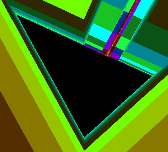
Sys: (3c) EMap, ((1+s*.01)*(y-sgn(x)*sqrt(abs(b*x-c))),(1+s*.01)*(a-x)), a = 4.800; b = 1.700; c = -.032; s = .600; This iteration is defined by: x <- (1+s*.01)* (y-sgn(x)*sqrt(abs(b*x-c))), y <- (1+s*.01)* (a-x). Parameters are: a = 4.800; b = 1.700; c = -.032; s = .600; Image 1: This is a time-scaled version of the vector field in the EMap view. The time-scaling parameter is s. Increasing s decreases the size of the black "prisoner" regions in the EMap image.
|
|
Sys: (3c) IMap0010, (y-sgn(x)*sqrt(abs(b*x-c)),a-x), a = 3.500; b = .125; c = .000; This iteration is defined by: x <- y-sgn(x)*sqrt(abs(b*x-c)), y <- a-x. Parameters are: a = 3.500; b = .125; c = .000; There are 3 seeds for the green, red and blue orbits in the lower left part of the image. They are visible as small black dots. Image 1: Three orbits in the IMap view, each with 10,000 t-steps. Watch the orbits mix. Image 2: First the green orbit extended 5 times. Image 3: Then the red orbit extended 5 times. Image 4: Then the blue orbit extended 5 times.
|
|
Sys: (3c) IMap1100, (y-sgn(x)*sqrt(abs(b*x-c)),a-x), a = 1; b=1; c=0 This iteration is defined by: x <- y-sgn(x)*sqrt(abs(b*x-c)), y <- a-x. Parameters are: a = 1; b=1; c=0 ICs: (0,0) give a period-3 cycle of (0,0) -> (0,a) -> (a,a) -> (0,0) for a = b, c = 0 Image 1: The (x,y) view, Image 2: The 3D/(t,x) view. Image 3: The 3D/(t,y) view.
|
|
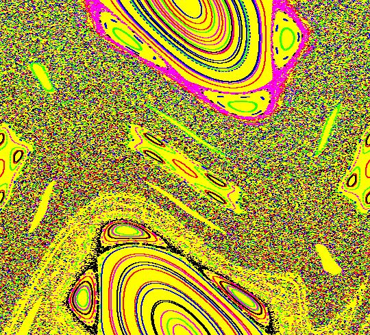
Sys: (3c) IMap1111, (y-sgn(x)*sqrt(abs(b*x-c)),a-x), a = 3.5; b = 1.2; c = 0; This iteration is defined by: x <- y-sgn(x)*sqrt(abs(b*x-c)), y <- a-x. Parameters are: a = 3.5; b = 1.2; c = 0; A total of 23 orbits have been started. There is a period 17 orbit in the outermost KAM island chain at (5.393583,4.371146) and a period 27 orbit in the next KAM island chain in at (4.720980,2.940080). Image 1: The period-17 orbit in the IMap view. Image 2: The period-27 orbit in the EMap view. Image 3: The various KAM island chains, with "Show 2D IMap Orbit Sequence" off. Conjecture: Every n-chain of KAM islands contains period n*m orbits, for m = 1, 2, 3, ... , out to the "dust" edge and the orbits starting the dust are chaotic. Try varying parameter b. For a reference on KAM theory and KAM islands, see.
|
|
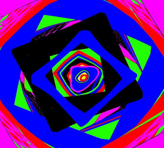
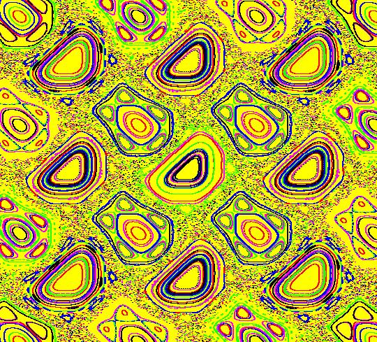
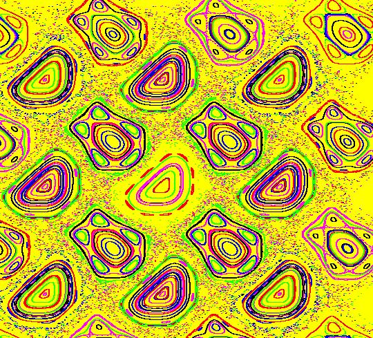
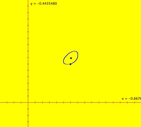
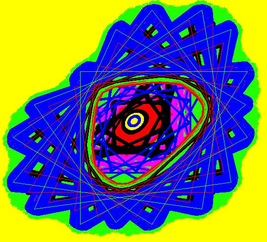
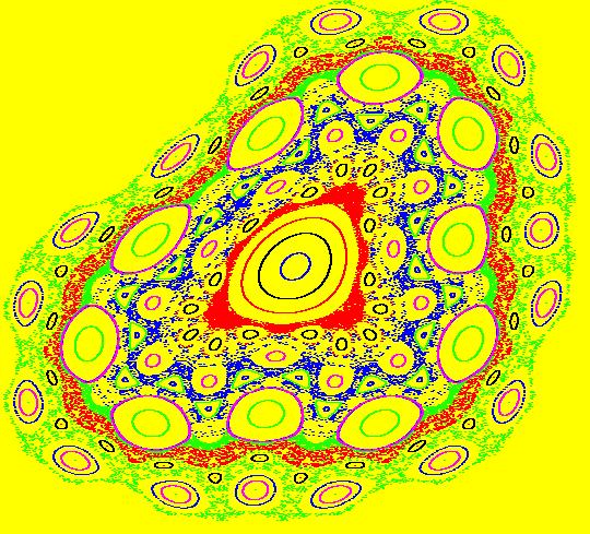
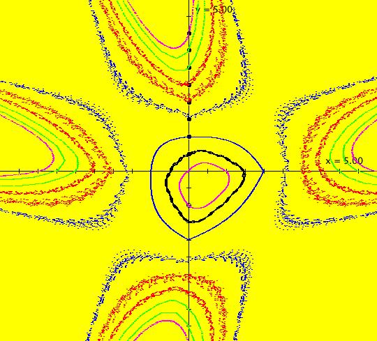
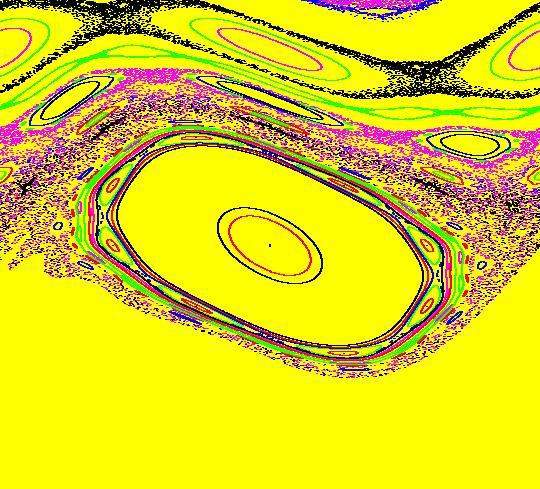
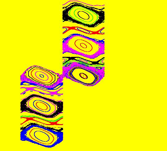
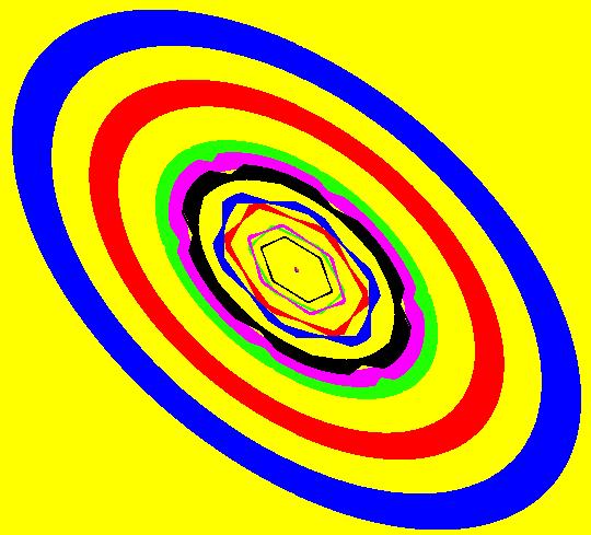
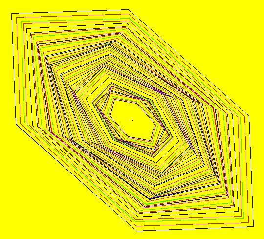
Sys: (3d) IMap0111, KAM islands (y-sgn(x)*sqrt(abs(b*x-c)),a-x), a = 3.5; b = 1.2; c = 0; This iteration is defined by: x <- y-sgn(x)*sqrt(abs(b*x-c)), y <- a-x. Parameters are: a = 3.5; b = 1.2; c = 0; Image 1: The rings of ellipses are KAM island chains. Each n-chain of KAM islands is filled with periodic orbits of period n*m, where m is a positive finite integer. Assuming that an orbit that starts in a KAM chain, stays in that chain, it is not difficult to see why this may be true. Computers use discrete number systems and discrete displays. Any iteration started in a particular KAM island belonging to an n-chain of KAM islands, will revisit the island after each group of n iterations. Suppose the (finite) number of points in the island is K. Since a computer can do more than K deterministic iterations, any iteration must eventually (in n*m steps for some m) return to a point that has already been visited. The regions between KAM islands contain chaotic orbits as well as more KAM island chains. In the small 7 island chain near the center of the image, there is an orbit of period 7 at (x,y) = (-2.764689,6.264689). Start a Flow animation to see the period-7 orbit. Another way to see the period-7 orbit is to switch to the EMap view. Image 2: EMap view, zoomed in, with a period-7 orbit shown. Zoom in 8X and start a periodic orbit near the period-7 orbit. Note that the orbit has a period divisible by 7.
|
|
Sys: (4a) IMap0100, (10*x%1), left shift map This is a simple example of an iterative map that is easy to analyze mathematically but impossible to analyze using any computer computation! The difficulty arises because: (a) computer computations can only use a finite subset of the infinite real number system and (b) exact conversions between base 10 and base 2 numbers in a finite number system are generally not possible. The iteration is defined by: x <- 10*x%1. It simply shifts the digits in the fractional part of x one place to the left and then discards the integer part of x. Begin by considering 0 < x0 < 1. If x0 is a rational number then it has a repeating decimal expansion. For example 47/123 = .38211 38211 38211 ... or 47/123 = .38211 with period-5. If x0 is irrational, the digits do not repeat. Mathematically it is easy to see that the iteration has an infinite number of periodic orbits, of all periods, as well as an infinite number of non-periodic orbits. Since for any periodic orbit starting at a rational number there are non-periodic orbits starting at irrational numbers arbitrarily nearby, the system is chaotic. See Chaos Theory To understand why viewing the periodic orbit by computing iterates is impossible, consider entering ICs: (t0,x0) = (0,.38211 38211 38211 38211). In the first place, the infinite decimal expansion of 47/123 cannot even be entered. We will always have some truncation error due to the 64 bit storage size defined for doubles in Java, or any other computer language. Furthermore, the base-10 to base-2 to base-10 conversion creates some error for the wrong number. Consider the blue orbit for x0 = 47/123. The rational number 47/123 gets truncated to 16 decimal digits and the last digit gets rounded up from 3 to 4 so at t = 0 p.x = 0.38211 38211 38211 4
The 1st iteration, at t = 1, is: p.x = 0.8211 38211 38211 40 The 2nd iteration is:
p.x = 0.211 38211 38211 3958 The last 4 digits became 3958 due to the base-10 to base-2 to base-10 conversion. The rest of the iterates follow. p.x = 0.11382113821139583 p.x = 0.13821138211395834 p.x = 0.38211382113958337 <- 1st cycle, t = 5 p.x = 0.8211382113958337 p.x = 0.2113821139583365 p.x = 0.11382113958336504 p.x = 0.13821139583365039 p.x = 0.38211395833650386 <- 2nd cycle, t = 10 p.x = 0.8211395833650386 p.x = 0.2113958336503856 p.x = 0.11395833650385612 p.x = 0.13958336503856117 p.x = 0.3958336503856117 <- 3rd cycle, t = 15 p.x = 0.9583365038561169 <- no more cycles p.x = 0.5833650385611691 p.x = 0.8336503856116906 p.x = 0.3365038561169058 p.x = 0.3650385611690581 <- t = 20 p.x = 0.6503856116905808 p.x = 0.5038561169058084 p.x = 0.03856116905808449 p.x = 0.3856116905808449 p.x = 0.8561169058084488 p.x = 0.5611690580844879 p.x = 0.6116905808448792 p.x = 0.1169058084487915 p.x = 0.16905808448791504 p.x = 0.6905808448791504 p.x = 0.9058084487915039 p.x = 0.05808448791503906 p.x = 0.5808448791503906 p.x = 0.8084487915039062 This next iterate, which has been computed incorrectly, is exact in base-2 p.x = 0.0844879150390625
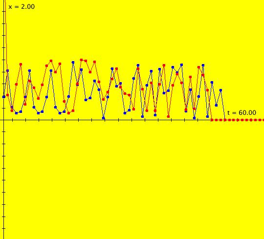
The rest of these 16-digit iterates have 0s at the end, so the iteration goes to 0 p.x = 0.844879150390625 p.x = 0.44879150390625 p.x = 0.4879150390625 p.x = 0.879150390625 p.x = 0.79150390625 p.x = 0.9150390625 p.x = 0.150390625 p.x = 0.50390625 p.x = 0.0390625 p.x = 0.390625 p.x = 0.90625 p.x = 0.0625 p.x = 0.625 p.x = 0.25 p.x = 0.5 p.x = 0.0 <- fixed point reached at t = 51 A java program that produces these numbers is: class ModTest { public static void main(String[] args) { double x = 47.0/123.0; for (int i = 0; i < 60; i++) { System.out.println(i+" "+x); x = 10*x%1; } } There is also no way to start at an irrational point. So - the computer reports that every orbit goes to the fixed point 0 while in reality only the x0 = 0 orbit goes to 0. Next try x0 = pi to 16 significant figures: 3.141 5926 5358 9793 The blue orbit is x0 = 47/123 and the red orbit is x0 = pi to 16 sig figs. On the computer, (t,x) goes to 0 for all t and all x. Mathematically only (t,0) orbits go to 0. Image 1: Computed (0,47/123) and (0,pi) orbits both go to 0. Image 2: All computed (t,x) orbits go to 0.
|
|
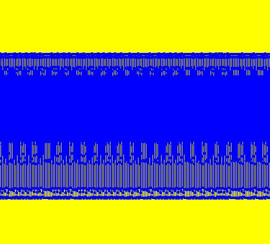
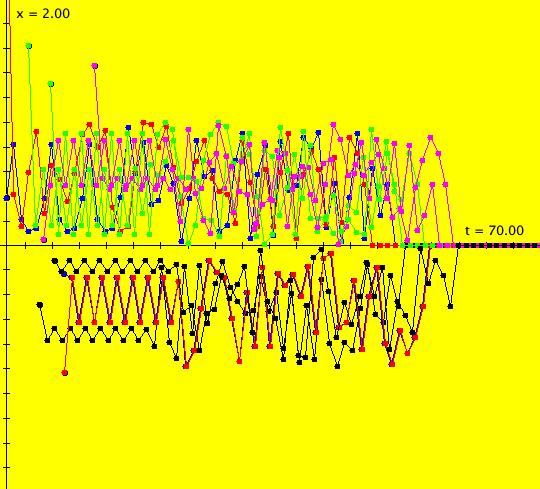
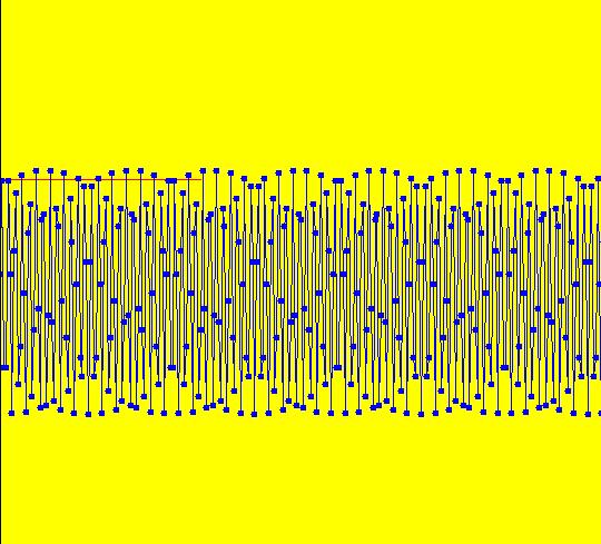
Sys: (4b) IMap0101 (x,x*y%1) (4a)'s bifurcation diagram This iteration is defined by: x <- x, y <- x*y%1. Here x plays the role of b in x <- b*x%1 i.e x is (4a)'s parameter. Image 1: The 2D bifurcation map of the 1D left shift map - as the computer sees it. In the computer, or computational, view of system (4b): (a) if b < -1 the system is chaotic and the amplitudes of the orbits are bounded in [-1,1], (b) if b = -1 all orbits are 2-cycles, (c) if -1 < b <= 1 all orbits go to 0, (d) if b > 1 the system is chaotic and the amplitudes of the orbits are bounded in [0,1] or in [-1,0]. The orbit in (4a), for b = 10 with ICs (t,x) = (0,47/123) = (0,.382113821138211...), corresponds to the orbit in this system, (4b), with ICs (x,y) = (10,.382113821138211...). To see this orbit clear the view, set vMax = 2, vMin - -2, hMin = -2 and hMax = 60 and get into the 3D/(t,y) view. Image 2: The 47/123 (4a) orbit in system's (4b) 3D/(t,y) view.
|
|
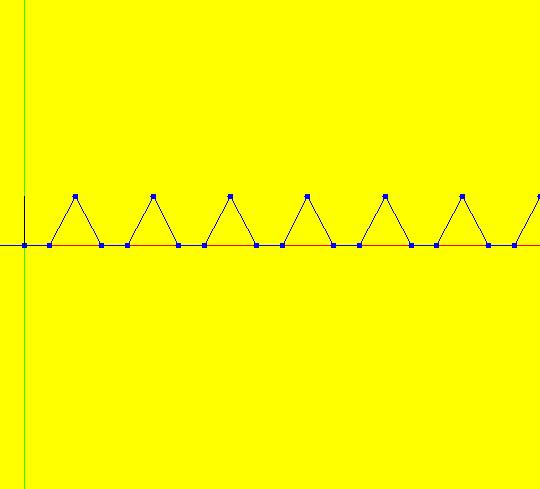
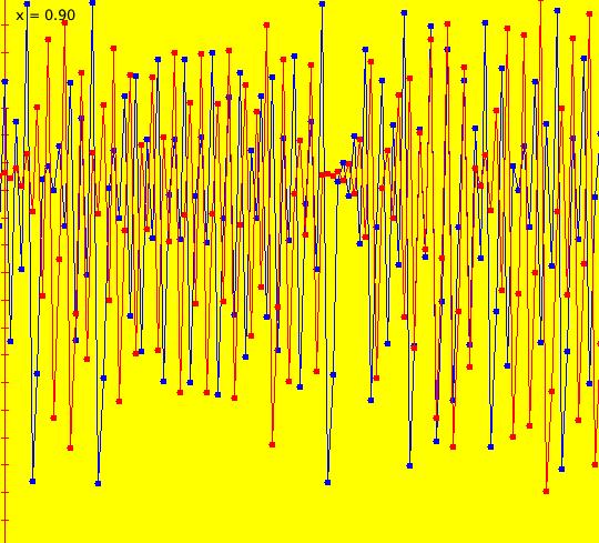
Sys: (5a) 1D IMap1100, (2*r*min(x,1-x)), r=.9 tent map This iteration is defined by: x <- 2*r*min(x,1-x). Parameters are: r=.9 Blue orbit: (t,x) = (0,.424528302). Red orbit: (t,x) = (0,.424528303). Image 1: A chaotic orbit. From Davies, "Exploring Chaos," p. 27, fig. 2.7. Decrease parameter r to .6 and watch what happens. Reference: tent map.
|
|
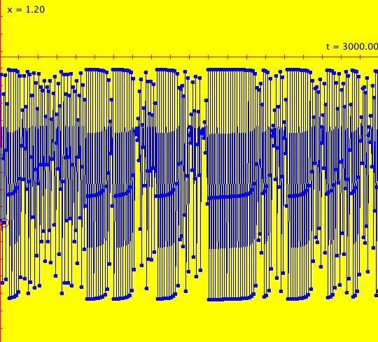
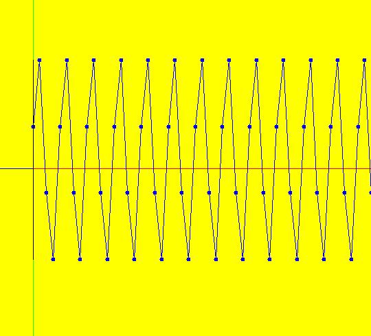
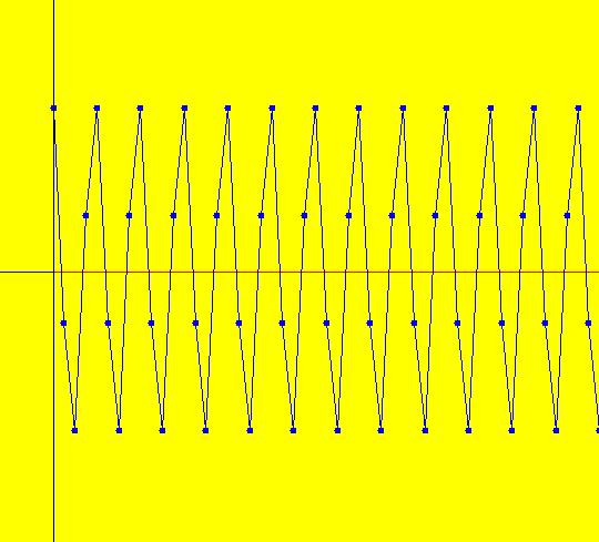
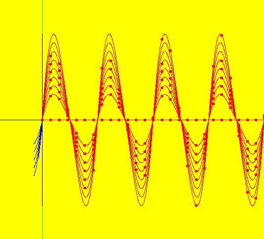
Sys: (5b) 2D IMap0001, (x,2*x*min(y,1-y)), tent bifurcation map This iteration is defined by: x <- x, y <- 2*x*min(y,1-y). Image 1: The bifurcation diagram for the tent map with three windows. The big window from x = .5 to about x = .7 is easy to see. There are also two narrower windows from x = .5 to about x = .589. Seeds for x <= .5 go to the fixed point y = 0. Seeds for .5 < x < ~ .677, give periodic orbits where the period is even. Seeds x > ~ .677 give chaotic orbits. Start a Flow to see the period-6098 orbit at (x,y) = (0.677020,0.564629). Image 2: The period-6098 trace after a Flow animation.
|
|
Sys: (5c) 2D EMapCT6 ((1+s*.1)*x,(1+s*.1)*2*x*min(y,1-y)), s = .700; This iteration is defined by: x <- (1+s*.1)*x, y <- (1+s*.1)*2*x*min(y,1-y). Parameters are: s = .700; Image 1: EMap of time-scaled tent map bifurcation diagram, (5b), w/CT 6.
|
|
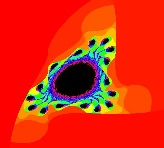
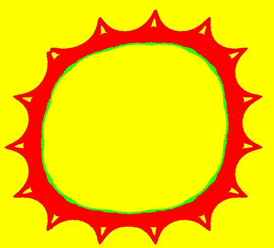
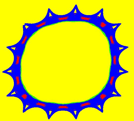
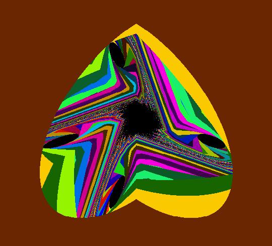
Sys: (6) Lozi EMapCT2 (1-a*abs(x)+b*y,x), a = 1.800; b = .600; This iteration is defined by: x <- 1-a*abs(x)+b*y, y <- x. Parameters are: a = 1.800; b = .600; Image 1: This EMap view is a "Julia" set of the 2D2P (2 Dimension, 2 Parameter) Lozi system.
|
|
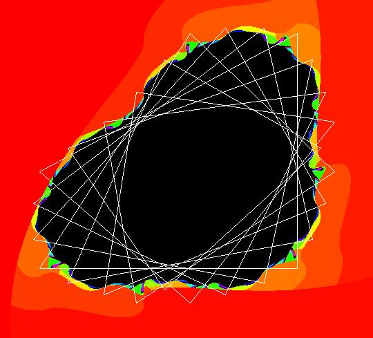
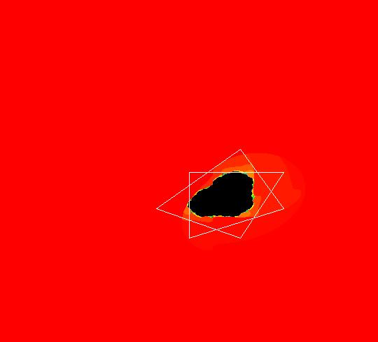
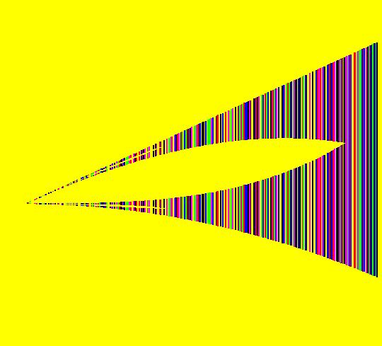
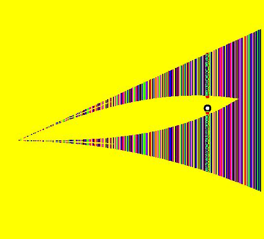
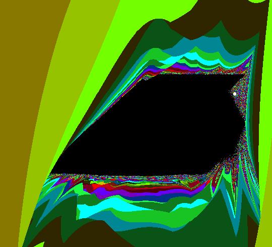
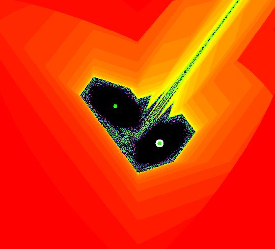
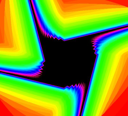
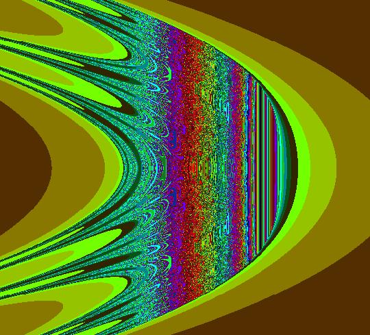
Sys: (6) Lozi EMapCT2 (x,y,1-x*abs(z)+y*w,z) This 4D system is the bifurcation diagram for the 2D2P Lozi system: x <- 1-a*abs(x)+b*y, y <- x. In the 4D system, x plays the role of parameter "a" and y plays the role of parameter "b" in the 2D2P Lozi system. The 4D system of odes, shown in the EMap view, is defined by the equations: dx/dt = x, dy/dt = y, dz/dt = 1-x*abs(z)+y*w, dw/dt = z. Image 1: This EMap view is the "Mandelbrot" set for the 2D2P Lozi system. The white dot is at (x,y) = (1.8,.6). The (x,y) points just outside of the black area (prisoner set) correspond to (a,b) pairs that give interesting looking "Julia" sets. The values (x,y) = (a,b) = (1.8,.6) are used in the previous system. You need to turn on "Show 2D IMap Orbit Sequence" to see where (1.8,.6) is.
|
|
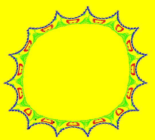
Sys: (6) Lozi EMapCT5 (1-a*abs(x)+b*y,x), a = .500; b = 1.100; This iteration is defined by: x <- 1-a*abs(x)+b*y, y <- x. Parameters are: a = .500; b = 1.100; Image 1: A Lozi "Julia" set w/CT 5. Image 2: The same Lozi "Julia" set w/CT 9.
|
|
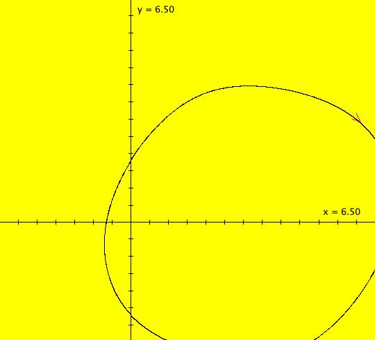
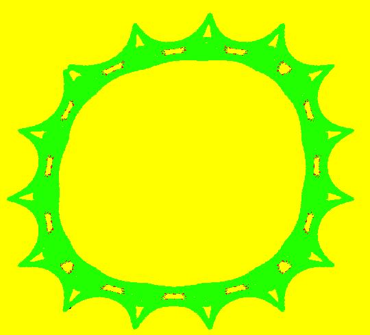
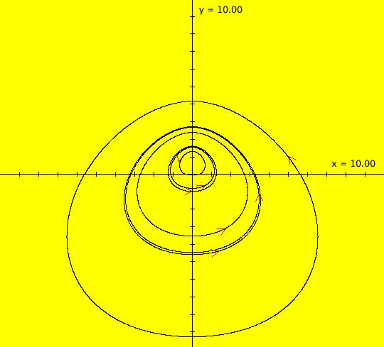
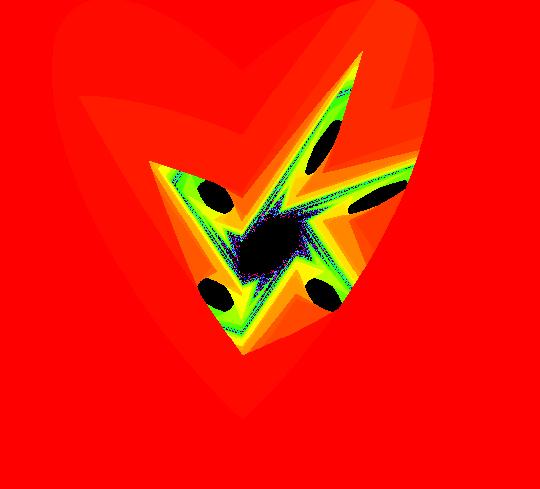
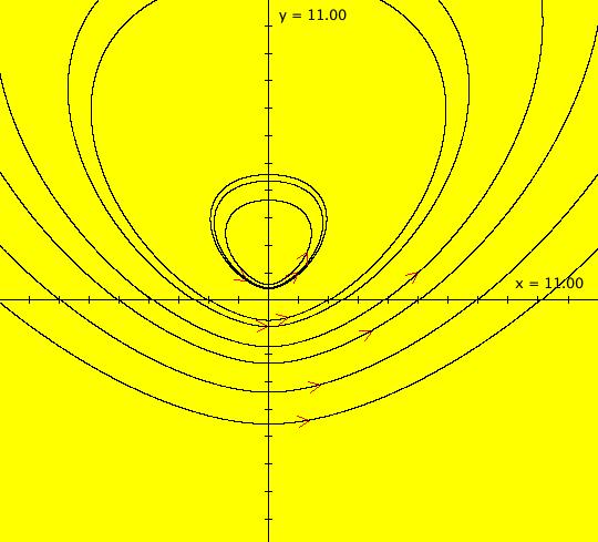
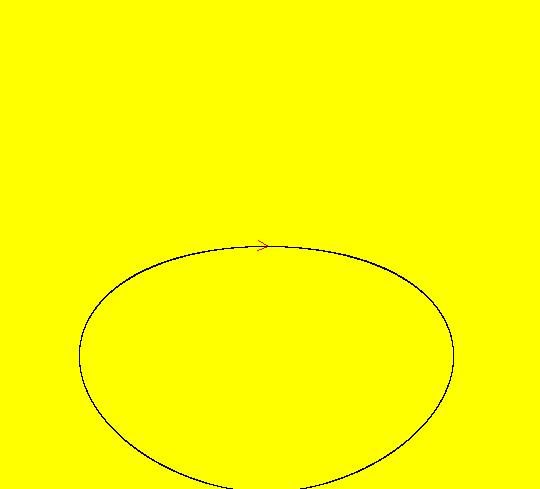
Sys: (6) Lozi EMapCT5 (1-a*abs(x)+b*y,x), a = .700; b = -1.000; This is an example of a system that is interesting as an Ode, an IMap and as an EMap. The IMap and EMap iterations are defined by: x <- 1-a*abs(x)+b*y, y <- x. Parameters are: a = .700; b = -1.000; EMap CT: 5 Image 1: Another EMap Lozi "Julia" set. See the Ode view. The system of odes is defined by the equations: dx/dt = 1-a*abs(x)+b*y, dy/dt = x. Parameters are: a = .700; b = -1.000; All Ode trajectories are cycles of period 6.707. There is a single Ode fixed point at (0,1). Image 2: The Ode view. Image 3: The IMap view.
|
|
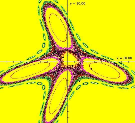
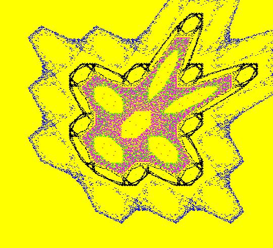
Sys: (6) Lozi IMap0011 (1-a*abs(x)+b*y,x), a = -1.000; b = -1.000; This is the Gingerbreadman version of the Lozi map. The iteration is defined by: x <- 1-a*abs(x)+b*y, y <- x. Parameters are: a = -1.000; b = -1.000; The orbit at p = (3.468635,-1.131313) has period 30. p is in a 5-chain KAM island and the orbit visits 6 points in each island in the chain. The orbit at (5,1) has per 19 and is in the 19-island black chain. Do a Flow to see the 19-island chain. All orbits, other than the fixed point at (1,1), in the single central KAM island have period 6. Orbits between KAM islands are chaotic. Image 1: IMap view. Image 2: EMap view w/CT 0. Image 3: EMap view w/CT 9. Image 4: Ode view. See Gingerbreadman map.
|
|
Sys: (6) Lozi IMap0011 L(a,b) (1-a*abs(x)+b*y,x), a=1; b=1 This iteration is defined by: x <- 1-a*abs(x)+b*y, y <- x. Parameters are: a=1; b=1 It is one form of the Lozi map. Another form is: x <- 1-a*abs(x)+y, y <- b*x. For a = 1, b = 1 there is a period-2 orbit at (x,y) = (1,-1). To see it, start an animation in the EMap view. Image 1: Just after a Flow animation in the EMap view For a = .9, b = 1 there is a period-2 orbit at (x,y) = (1.111111,-1.111111). To see this orbit, adjust "a" to .9 then start an orbit at (x,y) and run an animation.
|
|
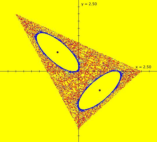
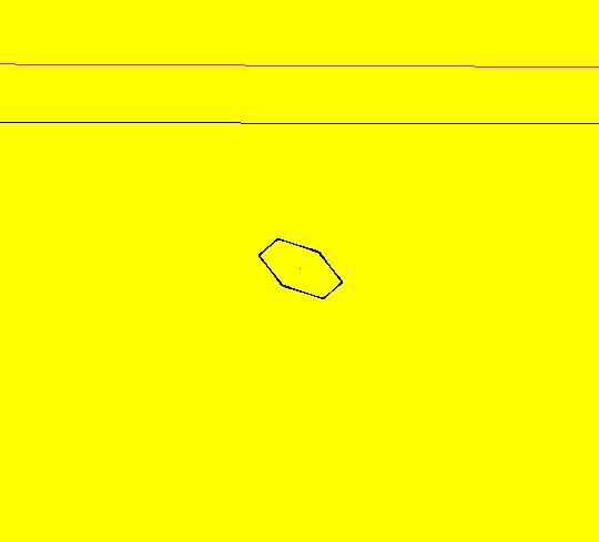
Sys: (6) Lozi IMap0100 L(a,b) (1-a*abs(x)+b*y,x), a = 1.500; b = 1.000; This iteration is defined by: x <- 1-a*abs(x)+b*y, y <- x. Parameters are: a = 1.500; b = 1.000; In the IMap view, orbits at (-2/3,2/3) and (2/3,-2/3) have period 2. There are 2 other chaotic orbits at (0,-.999990) and (0,-1.0000010) that create red and blue regions. Image 1: IMap view w/4 orbits. In the Ode view, (0,-1) is a fixed point. Image 2: Ode view. Image 3: EMap view w/CT 2.
|
|
Sys: (6) Lozi IMap1110 This iteration is defined by: x <- a+y-abs(x)/2, y <- -x. Parameters are: a=1 In the IMap view, there is a period 83 orbit at (0.007215,-0.334536). Image 1: A period-83 IMap orbit in the (x,y) view. Image 2: The same orbit in the 2D/(t,y) view with hMax = 300. Show that for a = .7 there is a period-4 orbit at (x,y) = (7,1.4). Find some more periodic orbits near (7,1.4). In the Ode view, all trajectories for this system are cycles with period 6.489 about the fixed point (0,-a). Image 3: Cycle w/period 6.489 in the Ode view. To see where the cycles come from, investigate the systems dx/dt = a+y-x/2, (6A) dy/dt = -x,
w/ICs (x,y) and dx/dt = a+y+x/2, (6B) dy/dt = -x w/ICs (-x,y).
|
|
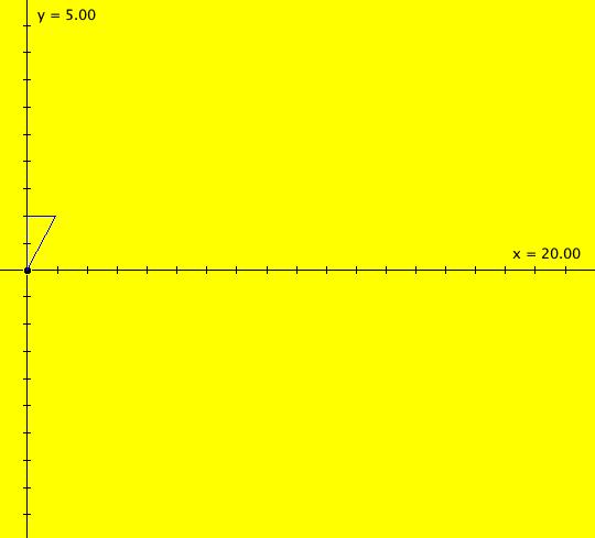
Sys: (6A) Lozi Ode (a+y-abs(x)/2,-x), a=1 This system of odes is defined by the equations: dx/dt = a+y-abs(x)/2, dy/dt = -x. Parameters are: a=1 ICs: (0,.5), (0,1), (0,1.5), ... , (0,4) Fixed point at (0,-1). In this Lozi system the abs(x) term combines the right and left halves of two linear systems to form a nonsmooth nonlinear system. One system is a cw out spiral system and the other is a cw in spiral system. For example, the right half of the outer trajectory in (6A) is the outer right half of the spiral in system (6B) and the left half of the outer trajectory in (6A) is the left half of the outer spiral in system (6C). Image 1: Ode view, cycles w/period 6.489 Image 2: Ode 3D/(t,x) view w/hMax = 4*6.489 = 25.956. Image 3: IMap view. Image 4: EMap view.
|
|
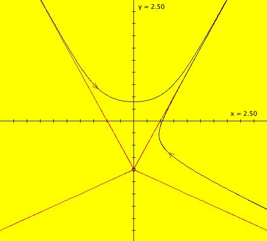
Sys: (6B) Lozi Ode right (a+y-x/2,-x), a=1 This system of odes is defined by the equations: dx/dt = a+y-x/2, dy/dt = -x. Parameters are: a=1 ICs: (0,4) cw spiral in with fixed point (0,-1) Image 1: The outer part of the trajectory for x>0 is the right half of the outer system (6A) trajectory.
|
|
Sys: (6C) Lozi Ode left (a+y+x/2,-x), a=1 This system of odes is defined by the equations: dx/dt = a+y+x/2, dy/dt = -x. Parameters are: a=1 ICs: (0,4) cw spiral out with fixed point (0,-1) Image 1: The outer part of the trajectory for x<0 is the left half of the outer system (6A) trajectory.
|
|
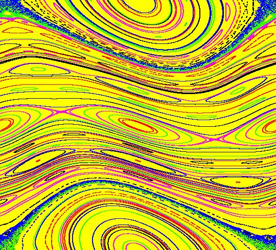
Sys: (7a) Standard IMap0111 ((x+y)%(2*pi)-pi,y+p*sin(x+y)), p=1 This iteration is defined by: x <- (x+y)%(2*pi)-pi, y <- y+p*sin(x+y). Parameters are: p=1 Reference: Lai, Ding and Grebogi, "Controlling Hamiltonian chaos," Physical Review E, vol 47, # 1, Jan. 1993. Image 1: A segment of the Standard map. The small black dot in the center of the image is an orbit of approximate period 6. To see the orbit, zoom in 3 times. The red dot in the center is a fixed point at (0, π). Note that the black orbit is smeared out a bit. This means that the orbit really has a period that is a multiple of 6. Turn on "Show 2D IMap Orbit Sequence" then, starting outside the black orbit, add some orbits near the black orbit. Image 2: Image 1 zoomed in 3X showing the period-6 orbit and the fixed point. Image 3: Image 1 zoomed out 2X showing how the main segment of the map, centered at (0, π), is just repeated forever in the y direction.
|
|
Sys: (7b) Standard IMap1111 ((x+y)%(2*pi)-pi,y+p*sin(x+y)), p=1 This iteration is defined by: x <- (x+y)%(2*pi)-pi, y <- y+p*sin(x+y). Parameters are: p=1 Near the fixed point (0, π) the orbits are approximately periodic with period 6. The orbit of the blue dot in the center of the image was created last and has period 1. With seed (x0,y0) = (0, π) x <- (0+ π)%(2* π)- π = 0 and y <- π+1*sin( π) = pi, so (0, π) is a fixed point of the IMap and the "period" of the orbit is 1, i.e. it takes just 1 step to get back to the seed. Image 1: Near (0, π). Image 2: Zoomed in 2X near (0, π).
|
|
Sys: (7c) Standard IMap0011 ((x+y)%(2*pi)-pi,y+p*sin(x+y)), p = 1.500; This iteration is defined by: x <- (x+y)%(2*pi)-pi, y <- y+p*sin(x+y). Parameters are: p = 1.500; See: D. A. Steck, Quantum Chaos, Transport, and Decoherence in Atom Optics, Ph.D. dissertation, 2001. Image 1: Image for K = p = .7 in Steck's dissertation, Appendix A, flipped about the y axis using the Lai/Ding?/Grebogi form of the "Standard" map. Image 2: K = p = 1.5 image.
|
|
Sys: (8a) 1D: (x^2+a), a = -1.76; IMap0100 This 1D iteration is defined by: x <- x^2+a. Parameters are: a = -1.76; Image 1: The seed is at (t,x) = (0,.5) and the period is 3. This example shows the relationship between: (8a) the 1D quadratic map and (8b) the 2D bifurcation diagram of (8a) and (8c) the EMap view of the time-scaled version of (8b) and (8d) the EMap view of the time-scaled version of the Henon map
|
|
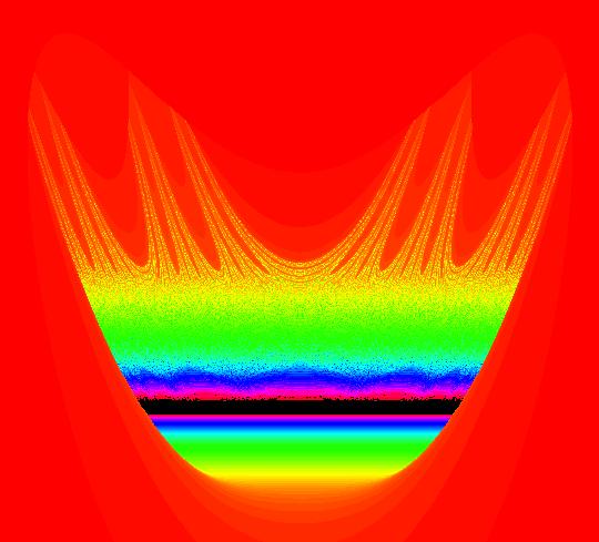
Sys: (8b) 2D: (x,x+y^2) IMap0011 This example contains many orbits so the image may take a while to appear. You will know that it has been completely rendered when the "EMap" button becomes enabled. The 2D iteration is defined by: x <- x, y <- x+y^2. It produces the bifurcation diagram for the 1D iteration: x <- a+x^2. The 1D system has many periodic orbits. In particular, it has periodic orbits with periods 1, 2, 3, 4 and 7. Can you find them? See: "Invitation to Dynamical Systems" by Edward R. Scheinerman, p. 151, Figure 4.29. Image 1: System (8a)'s bifurcation map.
|
|
Sys: (8c) ((1+.1*s)*x,(1+.1*s)*(x+y^2)), s = .580; EMapCT2 This iteration is defined by: x <- (1+.1*s)*x, y <- (1+.1*s)*(x+y^2). Parameters are: s = .580; Image 1: EMap CT: 2 This a time-scaled EMap version of (8b) which in turn is the bifurcation diagram for the 1D system (8a). If you rotate the vector field 90 degrees clockwise, then flip it about the y-axis, the system essentially becomes the Henon map. Also see Henon map. See system (8d), which is system "2D: EMap Henon map ver 2" in OdeFactory gallery "MapExs."
|
|
Sys: (8d) ((1+s*.01)*(1+y-.52*x^2),(1+s*.01)*y), s = 3.000; EMap This iteration is defined by: x <- (1+s*.01)*(1+y-.52*x^2), y <- (1+s*.01)*y. Parameters are: s = 3.000; Image 1: EMap CT: 0
| ||||||||||||||||||||||||