Click on an image to go directly to a system or scroll to see all of the systems in this gallery.
 |
 |
 |
 |
 |
 |
 |
 |
 |
 |
 |
 |
 |
 |
 |
 |
 |
 |
 |
 |
 |
 |
 |
 |
 |
 |
 |
 |
 |
 |
 |
 |
 |
 |
 |
 |
 |
 |
 |
 |
 |
 |
 |
 |
 |
 |
 |
 |
 |
 |
 |
 |
 |
 |
 |
 |
 |
 |
 |
 |
 |
 |
 |
 |
 |
 |
 |
 |
 |
 |
 |
 |
 |
 |
 |
 |
 |
 |
 |
 |
 |
 |
 |
 |
 |
 |
 |
 |
 |
 |
 |
 |
 |
 |
 |
 |
 |
 |
 |
 |
 |
 |
 |
 |
 |
 |
 |
 |
 |
 |
 |
 |
 |
 |
 |
 |
 |
 |
 |
 |
 |
 |
 |
 |
 |
 |
 |
 |
 |
 |
 |
 |
 |
 |
 |
 |
 |
 |
 |
 |
 |
 |
 |
 |
 |
 |
 |
 |
 |
 |
 |
 |
 |
 |
 |
 |
 |
 |
 |
 |
 |
 |
 |
 |
 |
 |
 |
 |
 |
 |
 |
 |
 |
 |
 |
 |
 |
 |
 |
 |
 |
 |
 |
 |
| OdeFactory Images and Annotations | |
|
An OdeFactory Slide Show Click on a slide to zoom in. Click "video" to see a video. |
View/Sys/Gal: Ode " Overview" in "VectorFields." ***** Overview ***** OdeFactory is a program used to study dynamical systems defined by vector fields of dimension less than or equal to four. The vector fields, when defined using explicit algebraic expressions, can be entered directly into the program as text strings in standard math syntax. The algebraic definition of the vector field, plus the display algorithms, generate the geometry of the system. There are also implicit ways to define vector fields. OdeFactory contains symbol manipulation algorithms that can construct AGF and quasiHamiltonian systems from user specified "generator" functions that end up among the solution curves. In this case, the algebraic generator functions create the vector field. This gallery demonstrates some indirect ways to define vector fields in OdeFactory. The sections are: AGFExs: 2D, uses complex and real lines ComplexFns: 2D, uses re(f(z)), im(f(z)) NonAutonToAutonExs: promote t, nD -> (n+1)D PMFn: pm(x) Post machine fn QuasiHamiltonian: 2D, uses fns of (x,y) TwoComplexLines: 2D AGF, uses 2 complex lines The program can also convert a 2D system from Cartesian coordinates to polar coordinates and a 2D two parameter system (2D2P) to a 4D zero parameter system (4D0P) that, in the 2D/(x,y) EMap view is the bifurcation diagram of the 2D2P system in the EMap view.
|
|
|
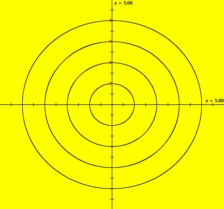
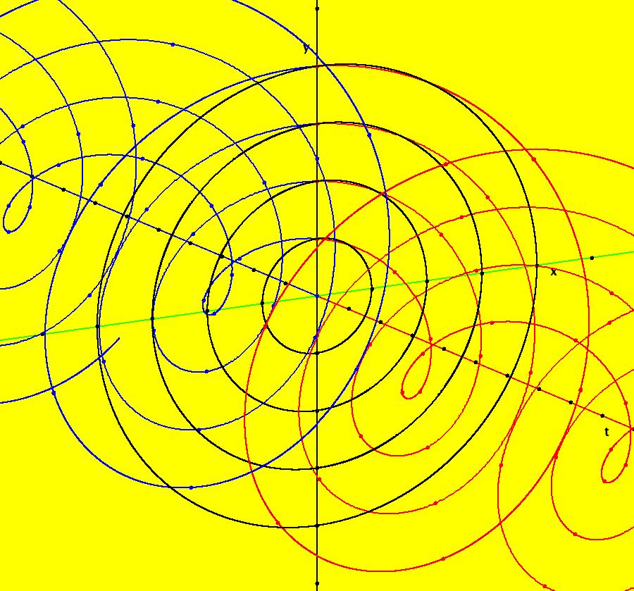
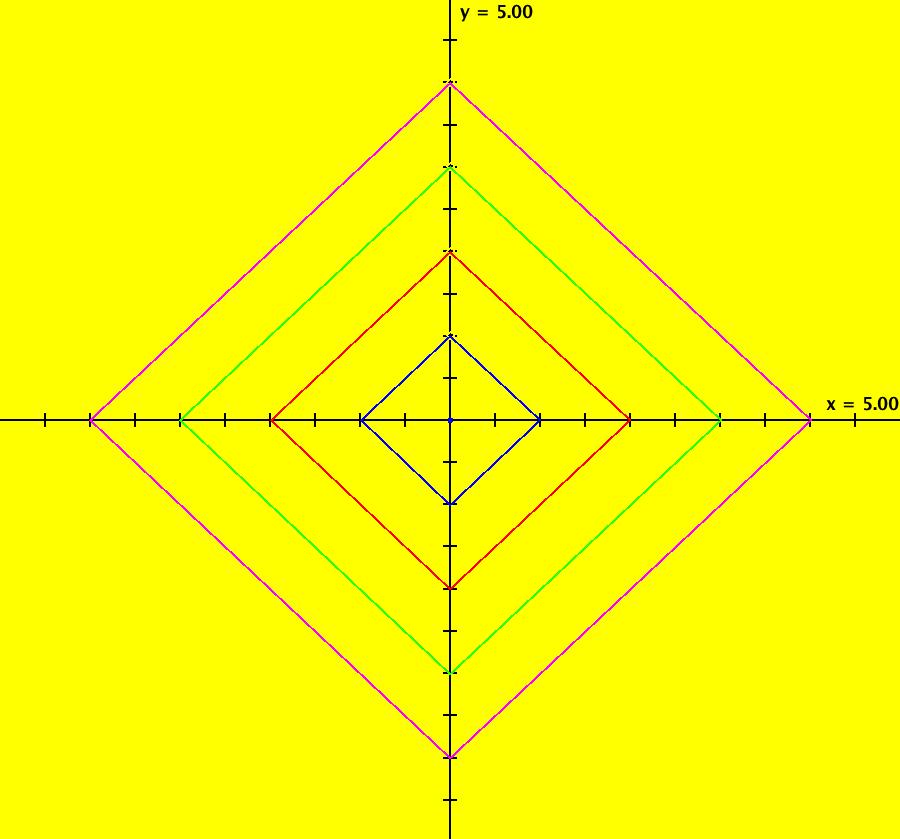
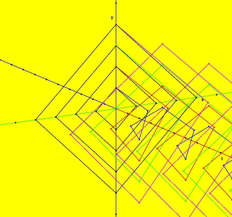
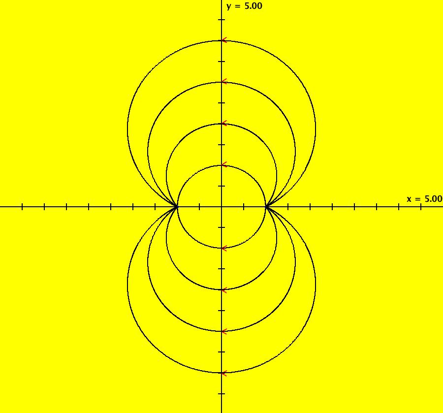
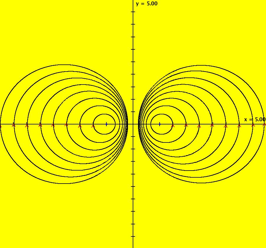
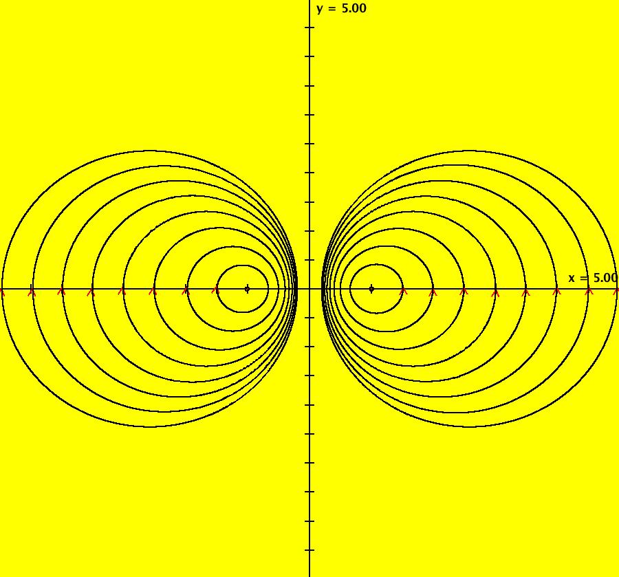
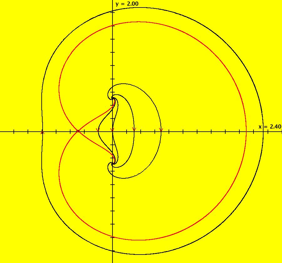
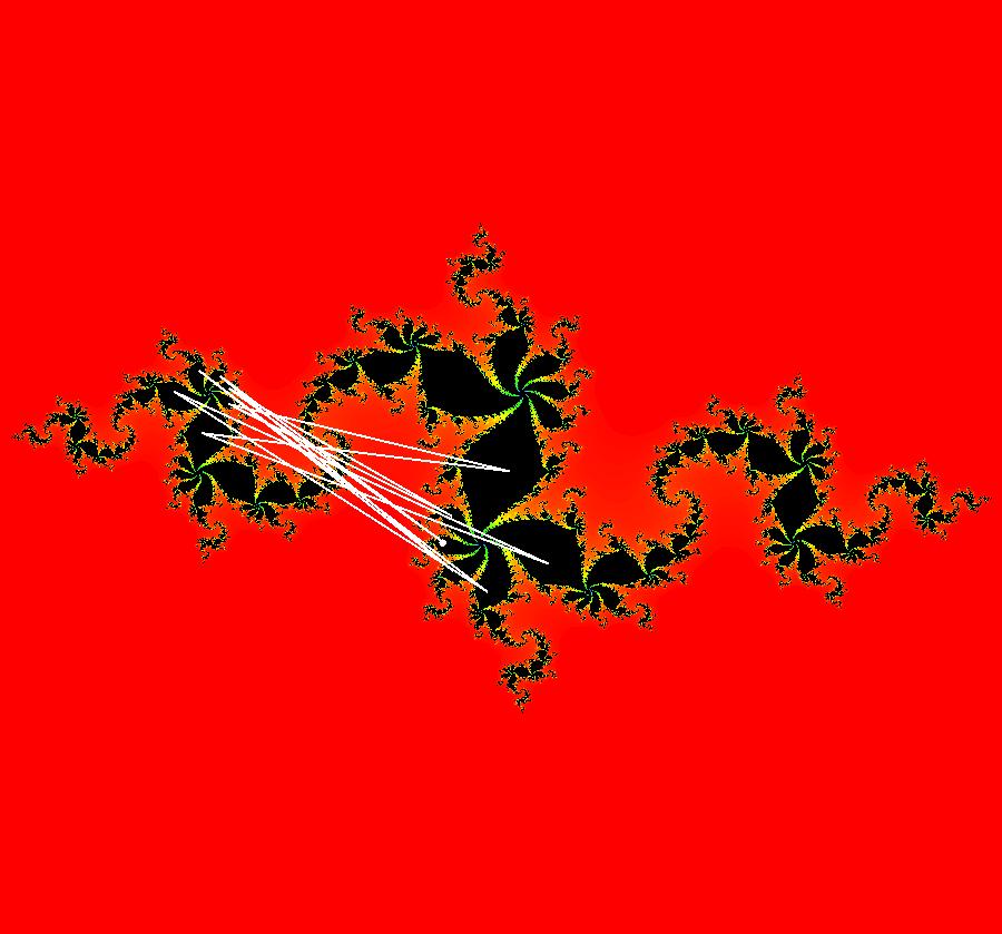
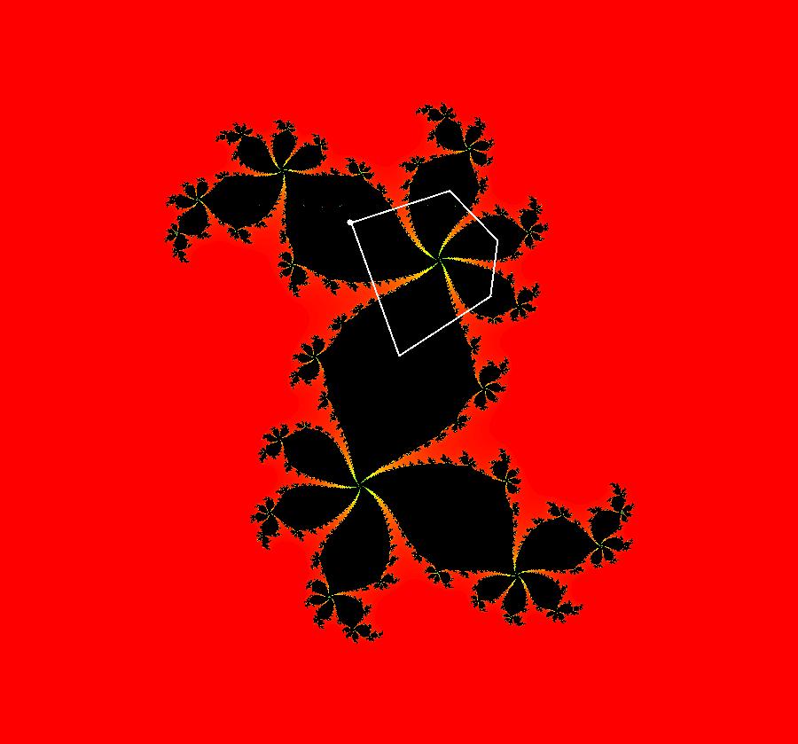
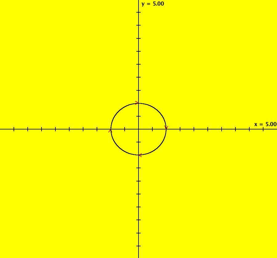
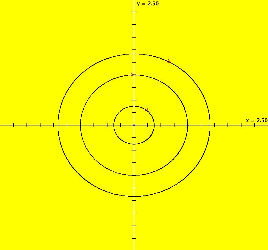
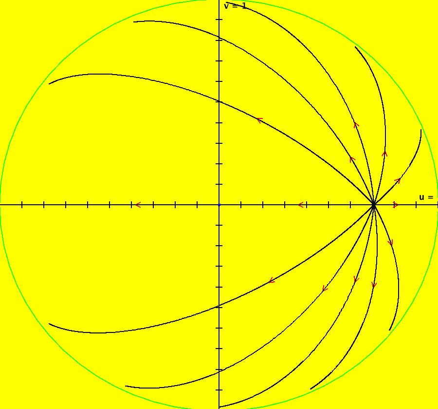
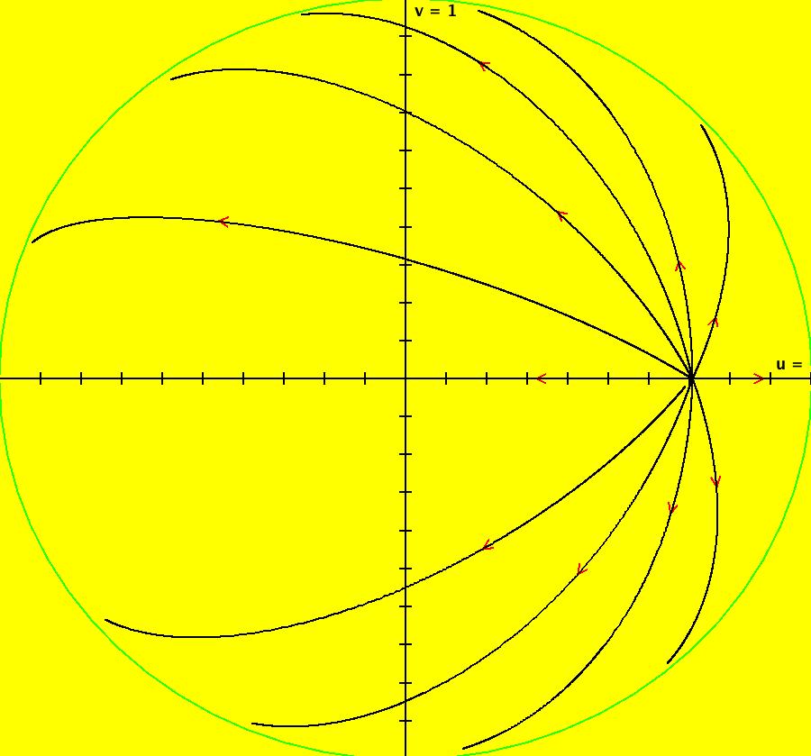
View/Sys/Gal: IMap "AGFExs: ***** Introduction *****" in "VectorFields." ***** Introduction ***** OdeFactory was originally written starting in 2009 to study 2D quasiHamiltonian Ode systems synthesized from real and complex lines called generators. The systems are called Algebraically Generated Flows, AGFs for short. See "AGFs" on the Help menu for further details. Selecting "center cw, λ = 1" with c = d = 0 in the "Define an AGF" window gives this first AGF which is generated by the complex lines: x+i*y = 0, λ1 = i, and it's complex conjugate, x-i*y = 0, λ2 = -i. The degree of the RHS of the system is: 1. The internal "dx/dt, dy/dt" form of the system is: dx/dt = y, dy/dt = -x Trajectories are circles centered at the origin. Solutions, for the ICs shown, are: x = y(0)*sin(t) and y = y(0)*cos(t). See the 3D/(t,x) and 3D/(t,y) views. Click on the blue dot at (0,0) to open a text-based controller for the complex generators parameters or shift-click to open a slider-based controller. Image 1: 2D Ode view of the colored vector field with 4 circular trajectories. The blue dot is the complex line. Image 2: 3D/(t,x,y) view of the Ode trajectories. Image 3: 2D IMap view with 4 square orbits. Image 4: 3D/(t,x,y) view of IMap orbits.
|
|
|
View/Sys/Gal: Ode "AGFExs: deg 1: 1 complex line" in "VectorFields." This AGF is generated by the lines: I[1]: x+i*y = 0, λ1 = i The degree of the RHS of the system is: 1. When you click "Insert Equations" the previous three lines are added to this Comments window and the internal dx/dt, dy/dt form of the system used by OdeFactory appears in the dx/dt, dy/dt fields as: dx/dt = (((y))), dy/dt = -((((x)))). Cartesian ICs: (x,y) = (0,1), (0,2), (0,3), (0,4) Applying WA to {{0,1},{-1,0}} gives eigenvalues i and -i. Image 1: Ode view.
|
|
|
View/Sys/Gal: Ode "AGFExs: deg 1: 1 complex line in Cartesian dx/dt, dy/dt form" in "VectorFields." This system of odes is defined by the equations: dx/dt = y, dy/dt = -x in the (t,x,y) coordinate system. This is the Cartesian form. Cartesian ICs: (x,y) = (0,1), (0,2), (0,3), (0,4) Clicking the Polar button gives (after simplifying using WA) the Polar form of this system as: dr/dt = 0, d θ/dt = -1 where r ∈ [0, ∞], θ ∈ [0,2 π]. Polar ICs: (r, θ) = (1, π/2), (2, π/2), (3, π/2), (4, π/2) In OdeFactory "dr/dt" is the "dx/dt" field and the "d θ/dt" is the "dy/dt" field. Image 1: Ode view.
|
|
|
View/Sys/Gal: Ode "AGFExs: deg 1: 1 complex line in Polar dr/dt. dθ/dt form" in "VectorFields." The Polar form of the system: dx/dt = y, dx/dt = -x, is dx/dt = (cos(y)*( ((((x*sin(y))))))+sin(y)*( -(((((x*cos(y)))))) )), dy/dt = (cos(y)*( -(((((x*cos(y)))))) )-sin(y)*( ((((x*sin(y)))))))/x. Image 1: Ode view in polar form using the "Polar" button. Applying WA to: simplify (cos(y)*( ((((x*sin(y))))))+sin(y)*( -(((((x*cos(y)))))) )) and simplify (cos(y)*( -(((((x*cos(y)))))) )-sin(y)*( ((((x*sin(y)))))))/x shows that the polar form of the system is really just: dx/dt = 0, read as "dr/dt = 0" dy/dt = -1, read as "d θ/dt = -1".
|
|
|
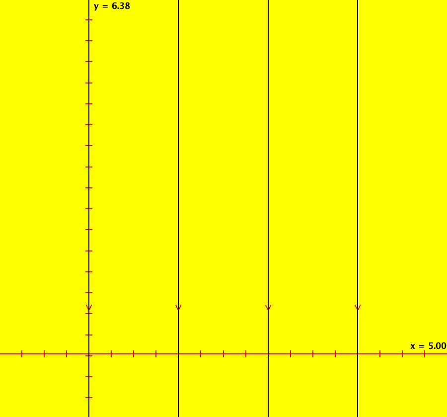
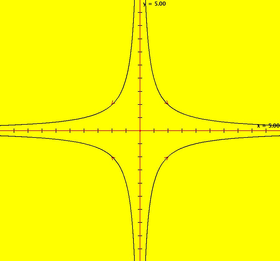
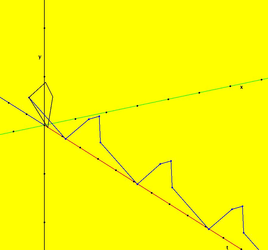
View/Sys/Gal: Ode "AGFExs: deg 1: 2 real lines" in "VectorFields." This AGF is generated by the lines: L[1]: y = 0, m = 0, λ1 = 1 L[2]: x = 0, m = inf, λ2 = -1 The degree of the RHS of the system is: 1. In dx/dt, dy/dt form the system is: dx/dt = x, dy/dt = -y In matrix form it is: dX/dt = A*X where A = {{1,0},{0,-1}} L[1] = y = 0 is the x axis and the 1st eigenvector of A is the unit vector in the x direction. The corresponding eigenvalue is 1. The flow is out on L[1]. L[2] = x = 0 is the y axis and the 2nd eigenvector of A is the unit vector in the y direction. The corresponding eigenvalue is -1. The flow is in on L[2]. Using WA on {x,y}=MatrixExp[{{1,0},{0,-1}}t].{a,b} gives the solution {x, y} = {a e^t, b e^(-t)}, where a = x(0), b = y(0). Select the "t" button to try the 3D/(t,x,y) extended phase space view. In the 3D view, click in the viewing area then select the (x,y) button. Also try the (t,x) and (t,y) buttons. Image 1: 2D Ode view. Image 2: 3D/(t,x,y) Ode view. In the 2D (x,y) view, shift-click on L[2] (the horizontal red line) to open a parameter controller. Increase the slope of the line. With the parameter controller still open get into the 3D/(t,x,y) view and adjust the slope of L[2].
|
|
|
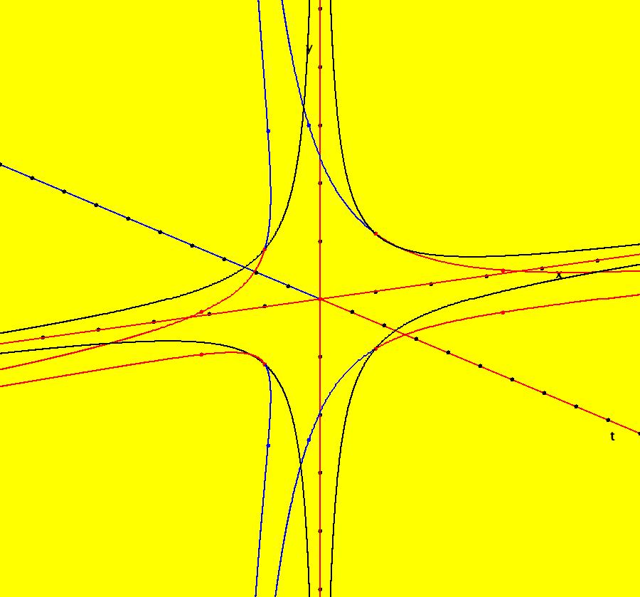
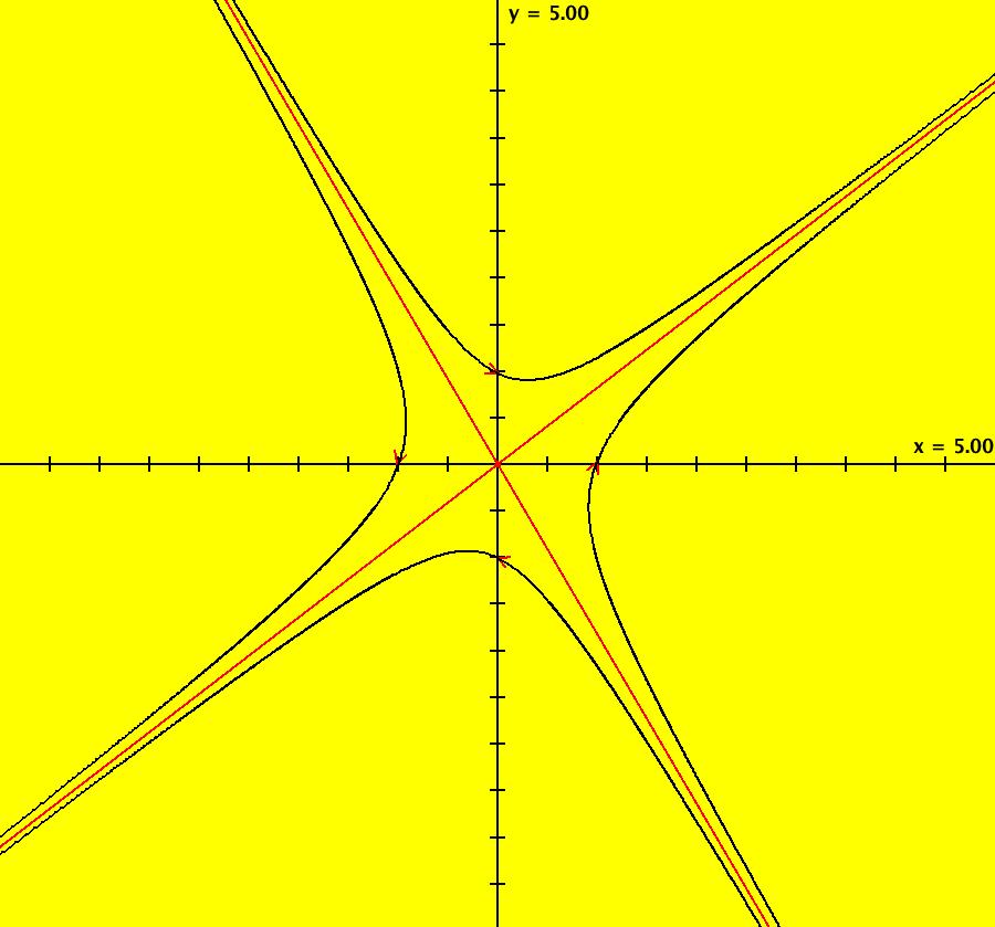
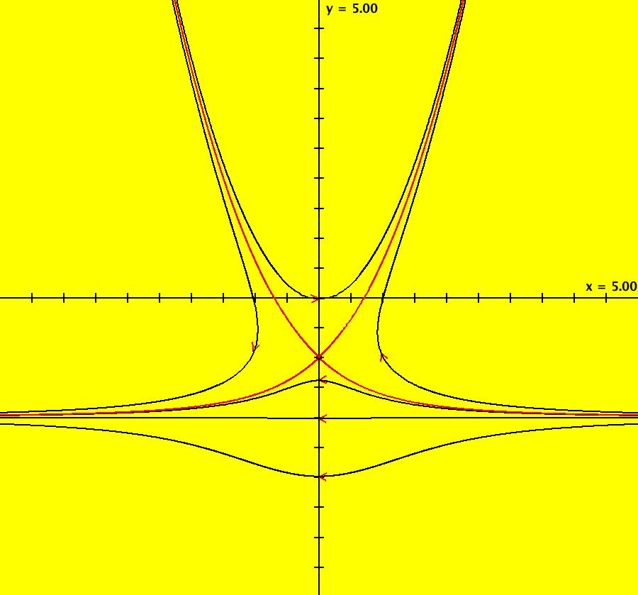
View/Sys/Gal: Ode "AGFExs: deg 1: dx/dt = x+2*y, dy/dt = 3*x-y" in "VectorFields." This system of odes is defined by the equations: dx/dt = x+2*y, dy/dt = 3*x-y Image 1: Ode view, red lines are the separatrices. WA applied to: {{1,2},{3,-1}} gives λ1 ~-2.64575, v1 ~{-0.548584, 1}, λ2 .64575, v2 ~{1.21525, 1} To corresponding AGF would have two linear generators with: m1 = 1/-0.548584 = -1.8228748 λ1 ~-2.64575 m2 = 1/1.21525 = .822876 λ2 .64575 The two linear generators would be the separatrices.
|
|
|
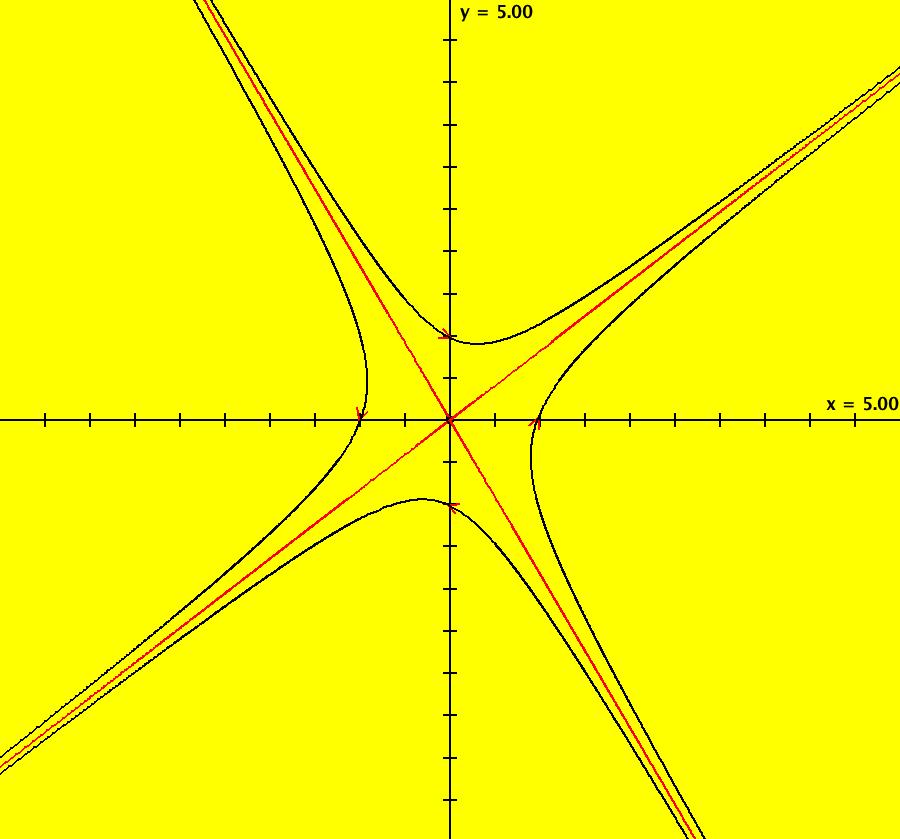
View/Sys/Gal: Ode "AGFExs: deg 1: dx/dt = x+2*y, dy/dt = 3*x-y as an AGF" in "VectorFields." This AGF is generated by the lines: L[1]: x+0.548584*y = 0, m1 = -1.822875, λ1 = -2.64575 L[2]: x-1.21525*y = 0, m2 = 0.822876, λ2 = 2.64575 The degree of the RHS of the system is: 1. L[1] and L[2] are the separatrices. Using WA, the dx/dt, dy/dt form of the system is: dx/dt ~ (-1.295*(0.635*x-0.772*y)+ 2.079*(0.877*x+0.481*y)), dy/dt ~ -((-2.361*(0.635*x-0.772*y)+ -1.711*(0.877*x+0.481*y))), which simplify to: dx/dt ~ x+2*y, dy/dy ~ 3*x-y. Image 1: Ode view, red lines are L[1] and L[2] which are also the separatrices.
|
|
|
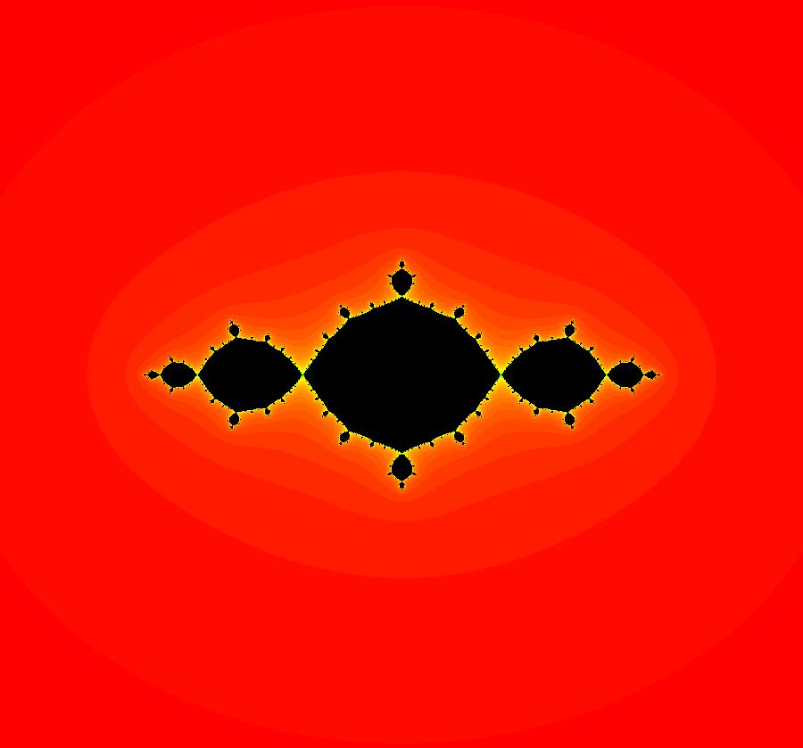
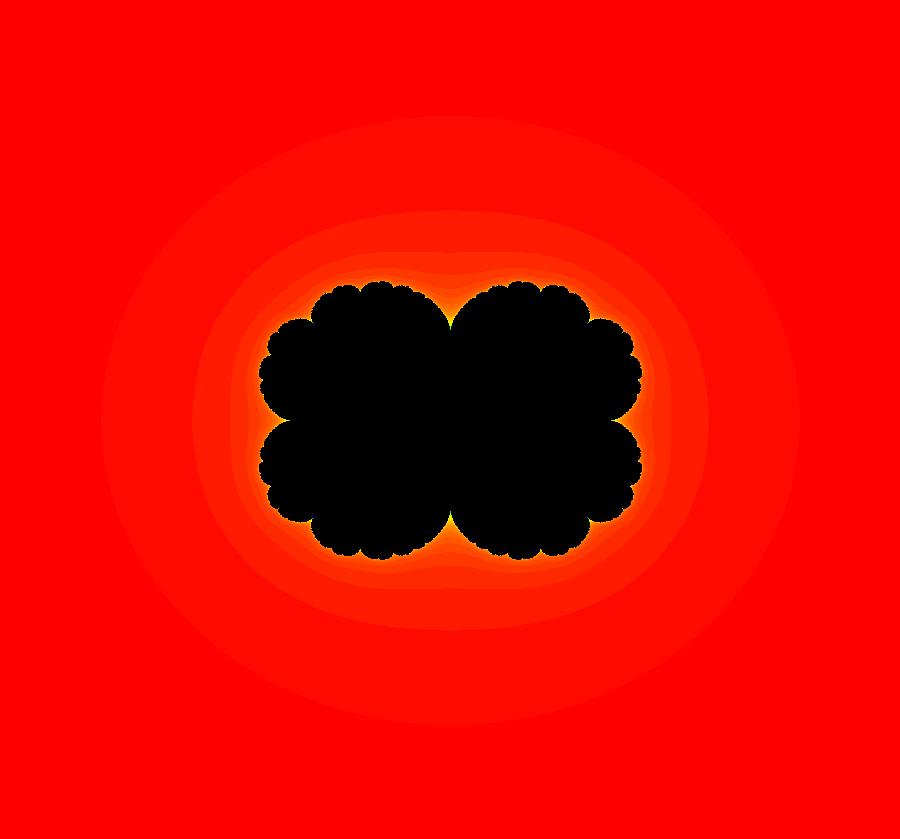
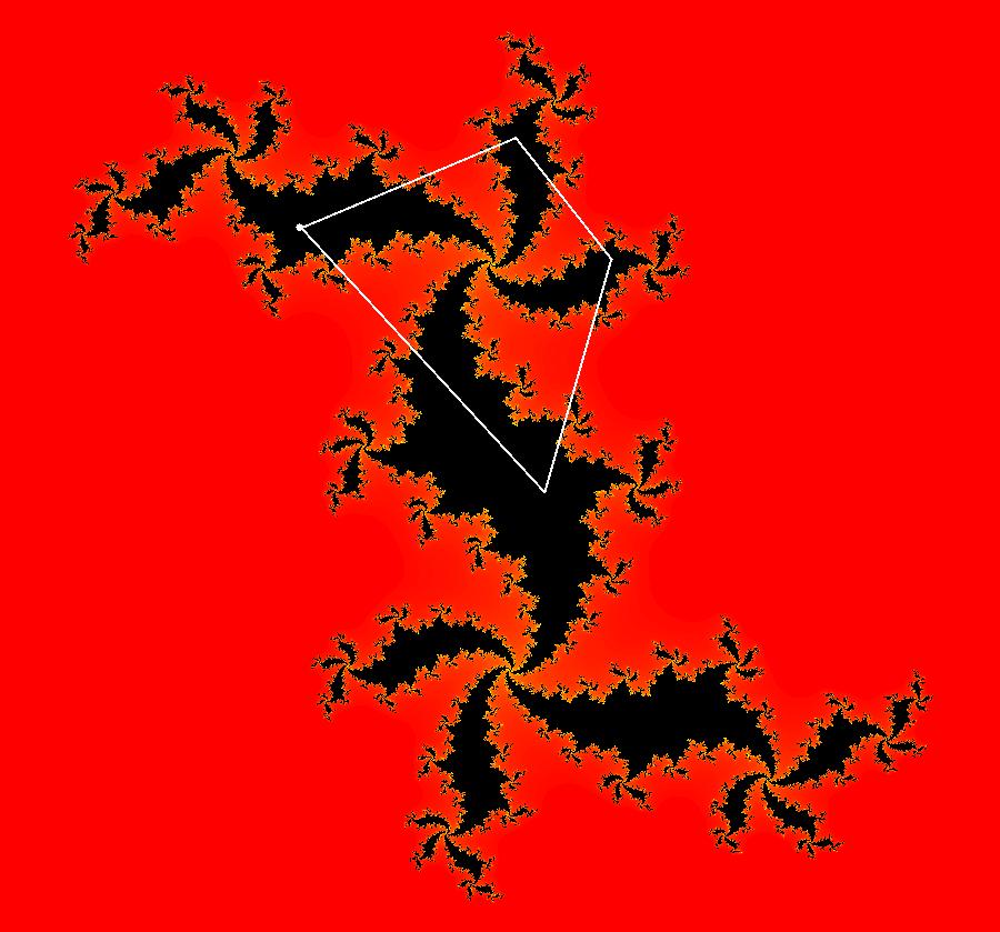
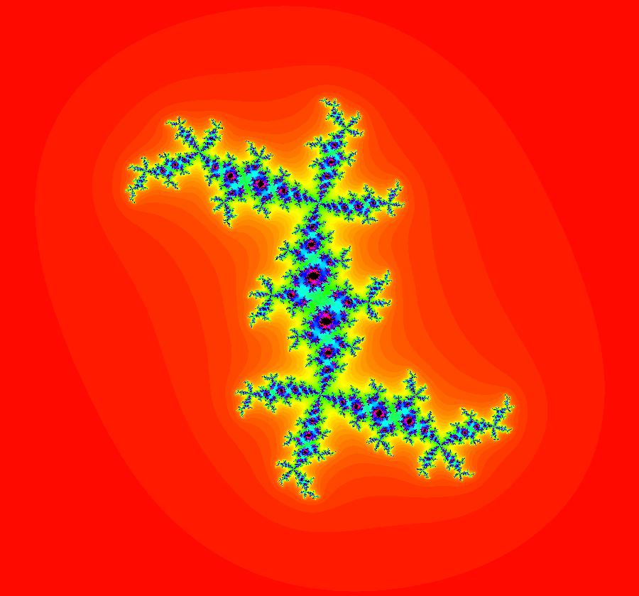
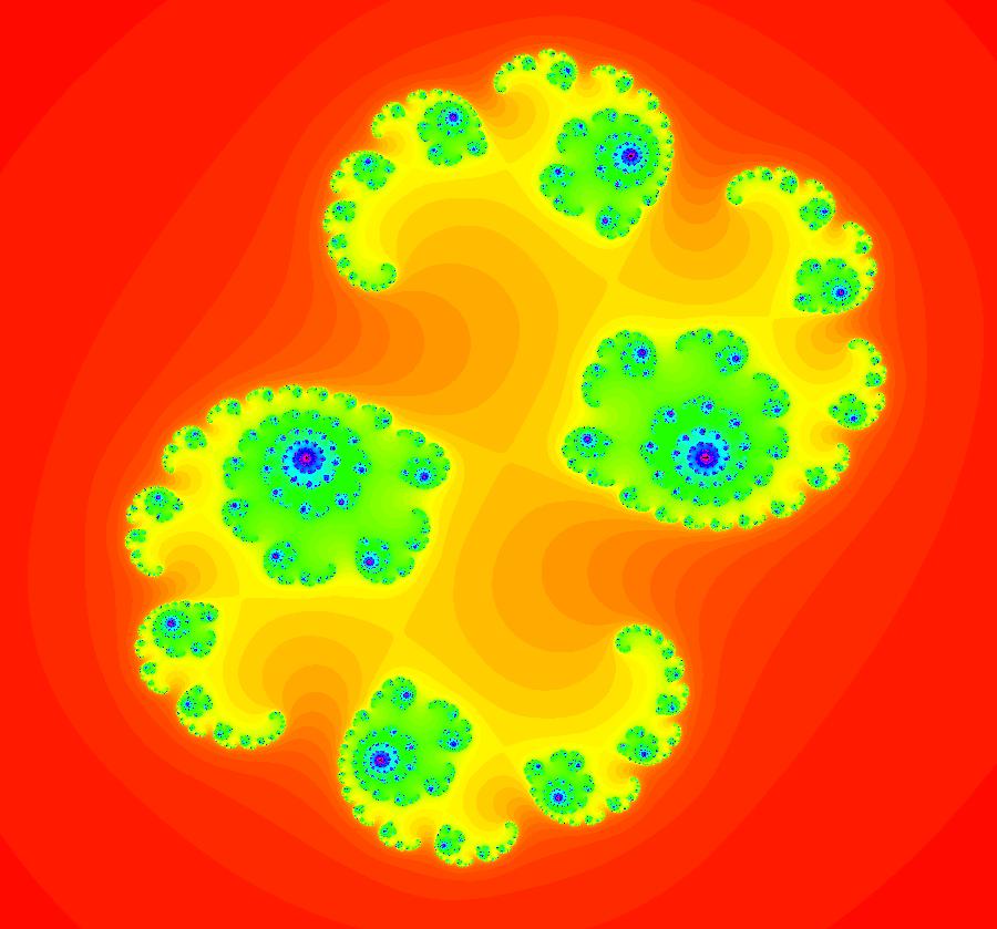
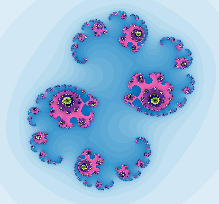
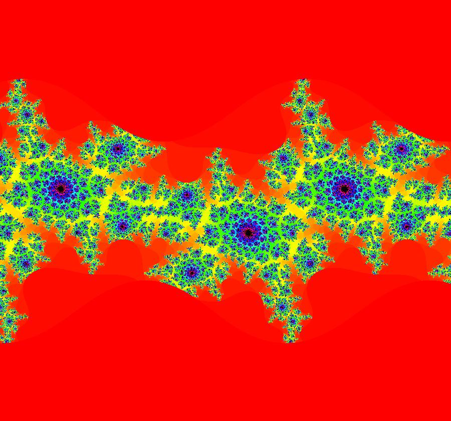
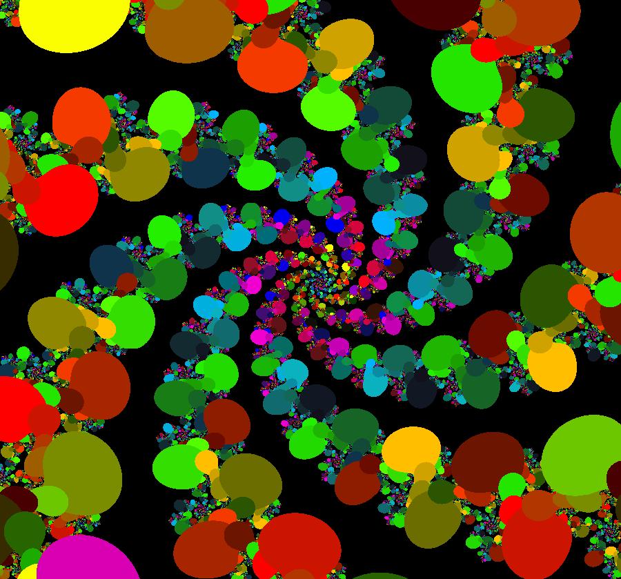
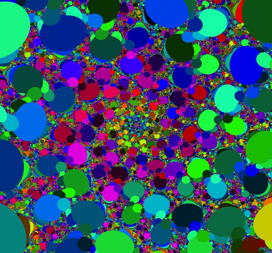
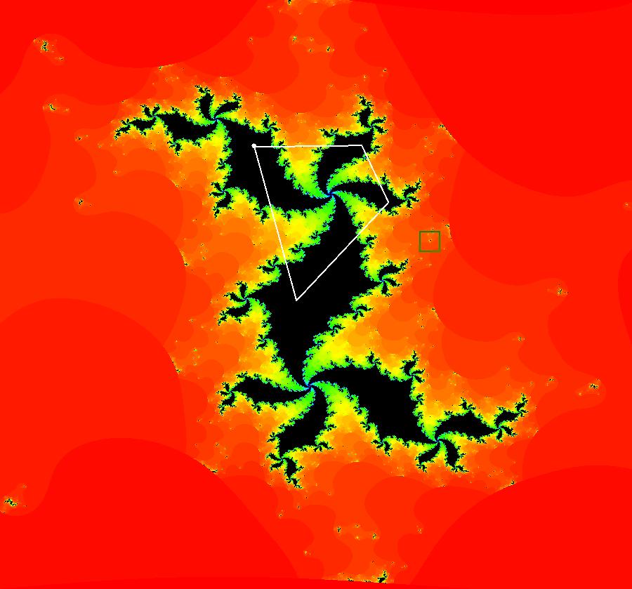
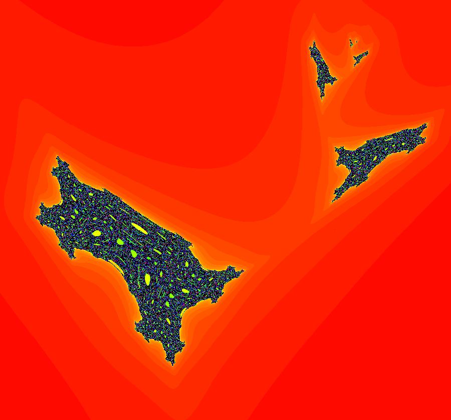
View/Sys/Gal: EMap "AGFExs: deg 2: 2 complex lines w/degree reduced by symmetry" in "VectorFields." This AGF is generated by the lines: I[1]: (x+0.3)+i*(y-0.66) = 0, λ1 = (-0.61-1.33*i) I[2]: (x-0.3)+i*(y+0.66) = 0, λ2 = (0.61+1.33*i) The degree of the RHS of the system would normally be 3 but due to symmetry it is reduced to 2. Using WA, the dx/dt, dy/dt form of the system is: dx/dt = 0.347369+1.0089*x^2-0.0066*x*y-1.0089*y^2 dy/dt = 0.400665+0.0033*x^2+2.0178*x*y-0.0033*y^2 The degree is 2 because of the symmetry: V(x,y) = V(-x,-y). The EMap view looks similar to a Julia set for the Mandelbrot map, z <- z^2+c but the Mandelbrot map has no x*y term in the x iteration and no x^2 or y^2 terms in the y iteration. Image 1: Ode view. Image 2: IMap view. Image 3: EMap view.
|
|
|
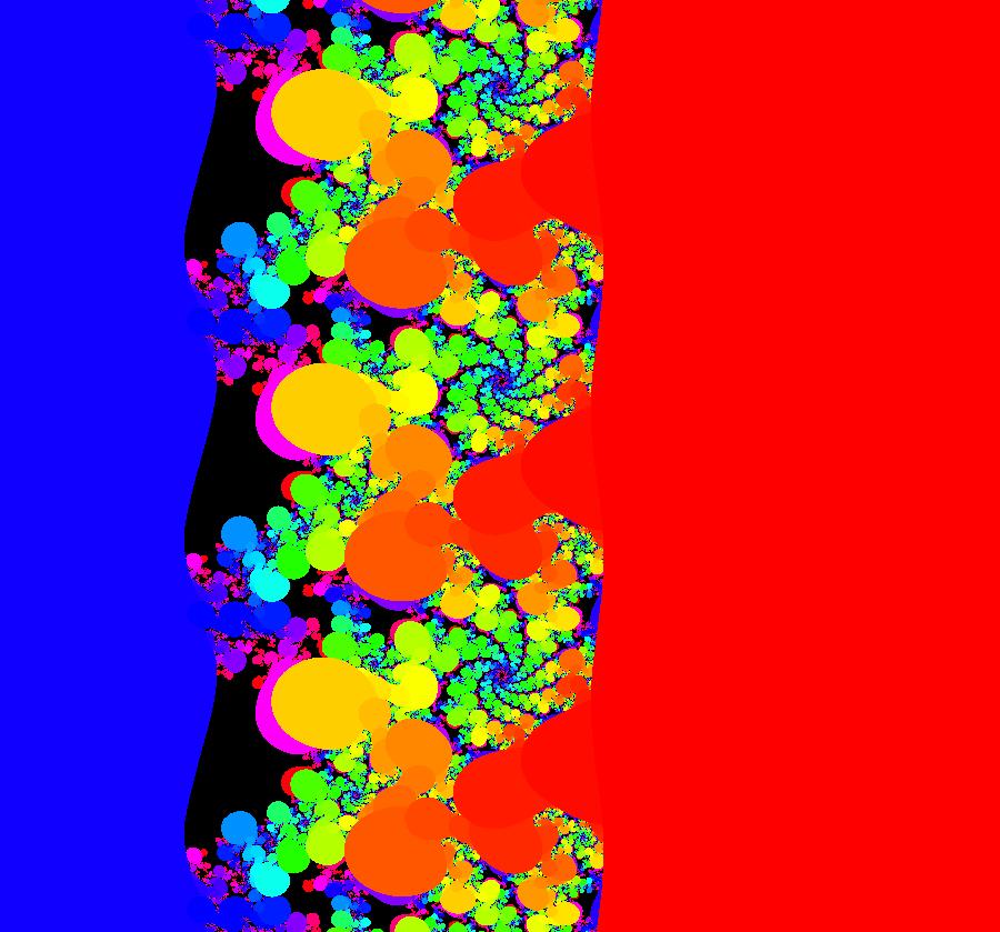
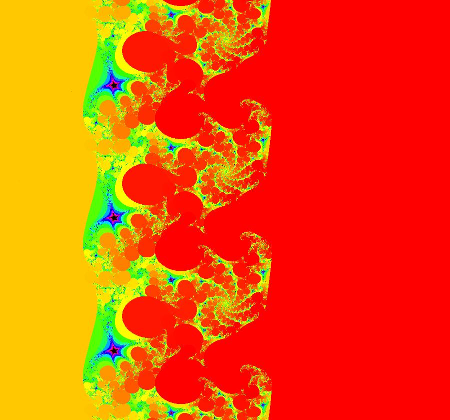
View/Sys/Gal: EMap "AGFExs: deg 2: 3 real lines" in "VectorFields." This AGF is generated by the lines: L[1]: (x+1)-y = 0, m1 = 1, λ1 = -1 L[2]: x+(y-1) = 0, m2 = -1, λ2 = -1 L[3]: y = 0, m3 = 0, λ3 = 1 The degree of the RHS of the system is: 2. Image 1: Ode view. Image 2: Ode view with the colored vector field on. Image 3: Ode R2+ view. Image 4: EMap view. The black region is a basin of attraction. The attractor is the point (0.414214,0). Shift-click on L[3] and increase the slope of L[3].
|
|
|
View/Sys/Gal: Ode "AGFExs: deg 2: 3 real lines, dx/dt, dy/dt form" in "VectorFields." This system of odes is defined by the equations: dx/dt = 0.499849-0.499849*x^2- 1.9994*y+1.49955*y^2, dy/dt = 0.999698*x*y. This is the same vector field as in the previous example. Image 1: Ode view with colored vector field on.
|
|
|
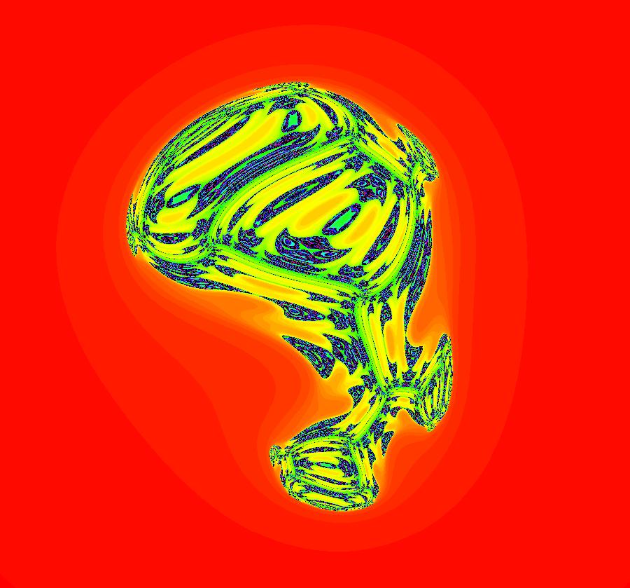
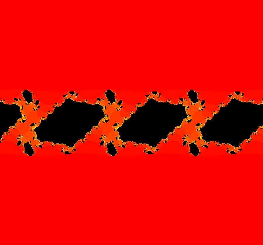
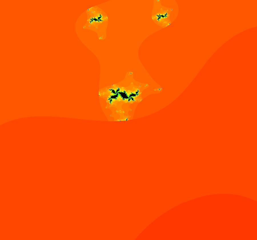
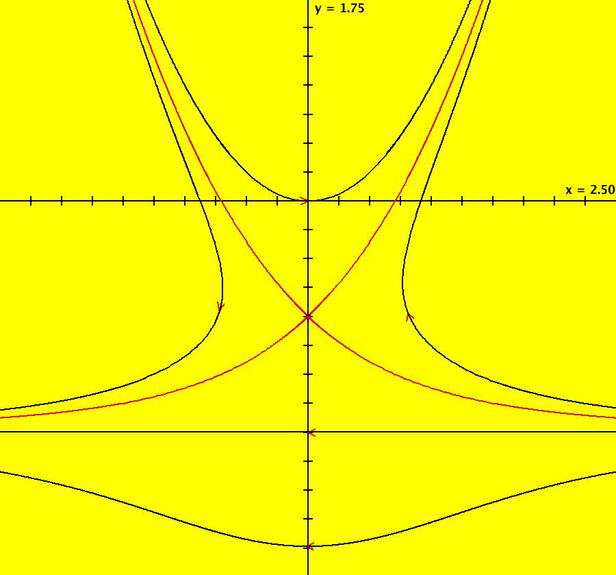
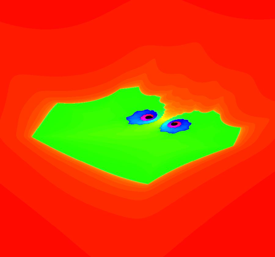
View/Sys/Gal: EMap "AGFExs: deg 2: parabola and line" in "VectorFields." This system of odes is defined by the equations: dx/dt = Q+P, dy/dt = 2*x*Q Parameters are: a = -2 Functions are: P = y-x^2, parabola through (0,0) Q = y-a, line parallel to y axis through y=-2 This is a Hamiltonian system with H = P*Q. dx/dt = ∂H/ ∂y = ∂P/ ∂y*Q+P* ∂Q/ ∂y = Q+P dy/dt = - ∂H/ ∂x = -( ∂P/ ∂x*Q+P* ∂Q/ ∂x) = 2*x*Q Image 1: Ode view. The parabola P and the straight line Q are the generators. They are among the solution curves. The solution curves are the level curves of H(x,y). Apply WA to: level curves of (y-x^2)(y+2). Image 2: EMapCT9 view shows a simple fractal center at about (-.6122449,-1.1450382). If the dx/dt and dy/dt fields are left empty when you update the system you get the more general quasiHamiltonian system: dx/dt = (b*Q+c*P), dy/dt = -(b*(-2*x)*Q) which is this Hamiltonian system when b = c = 1.
|
|
|
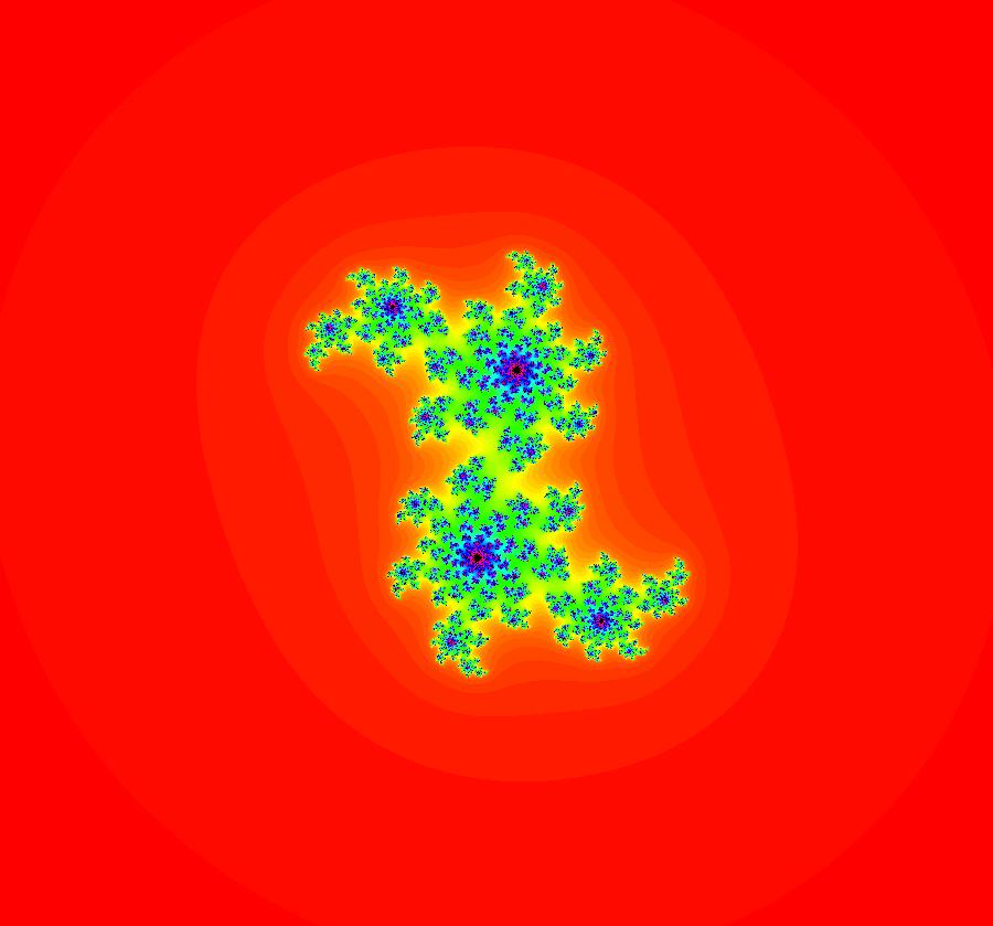
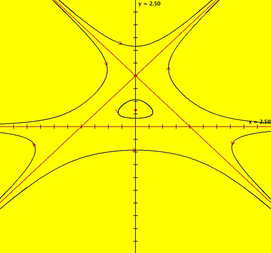
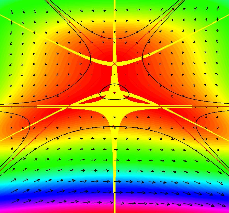
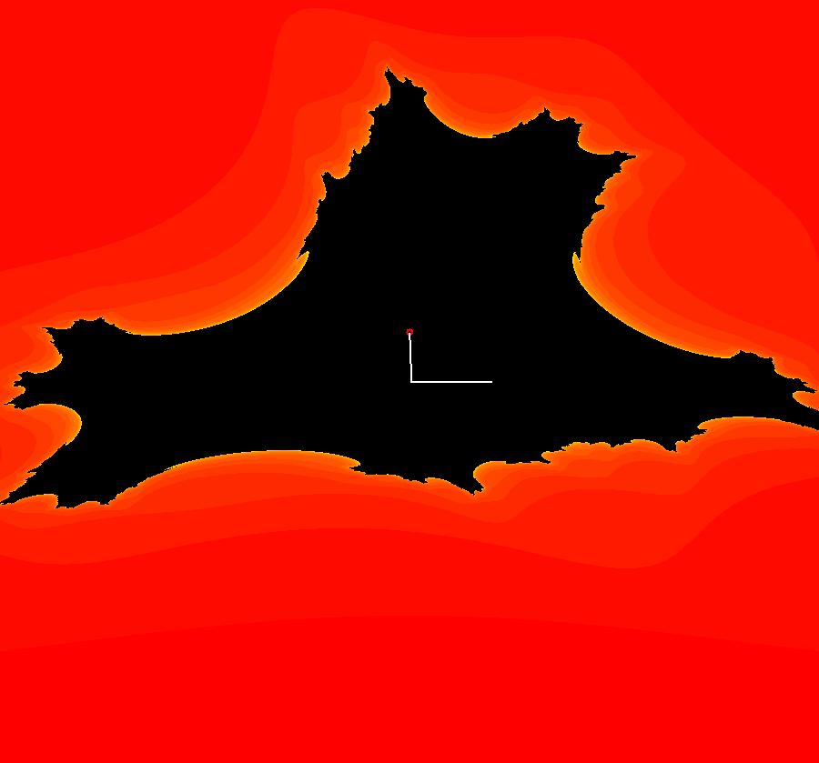
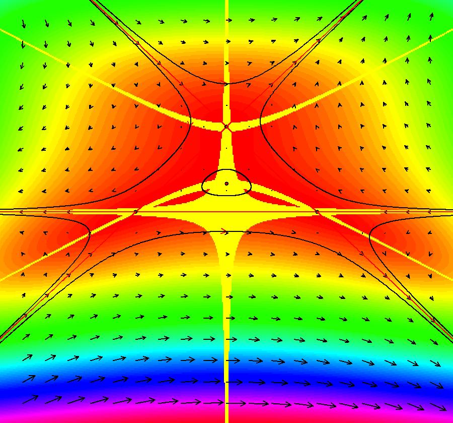
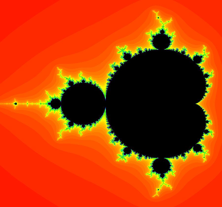
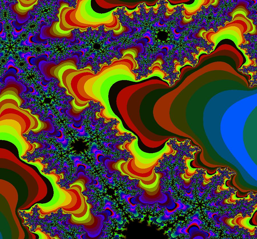
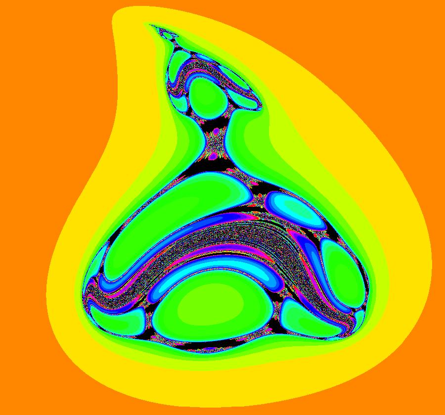
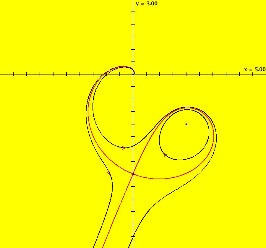
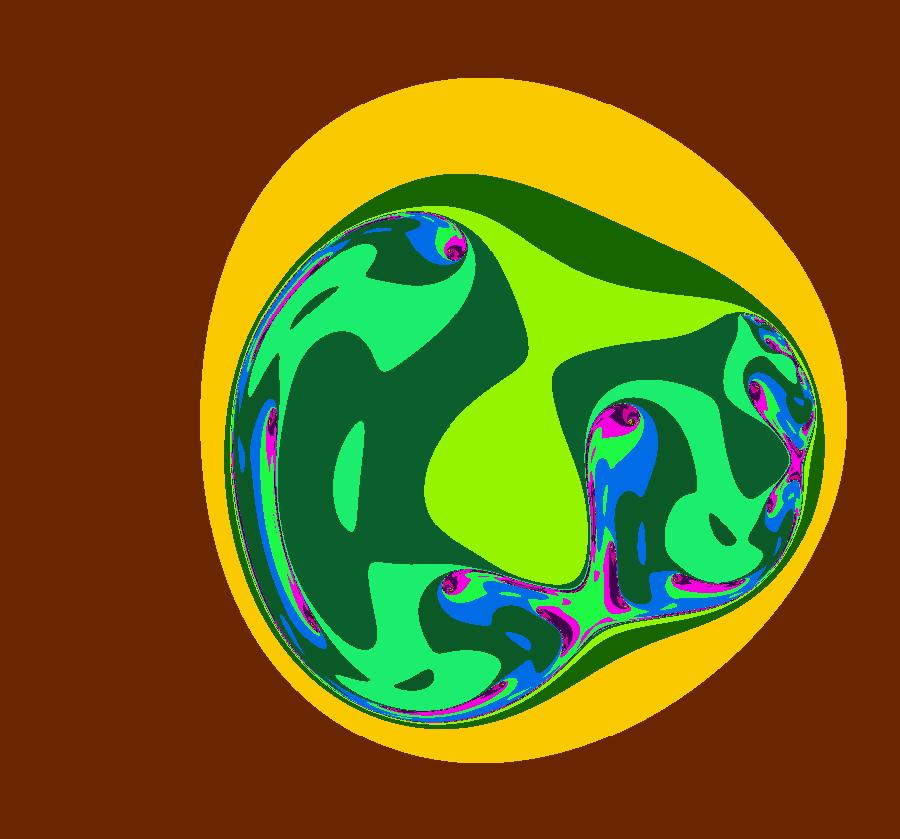
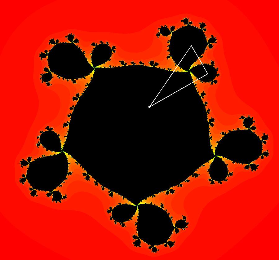
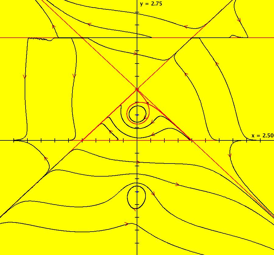
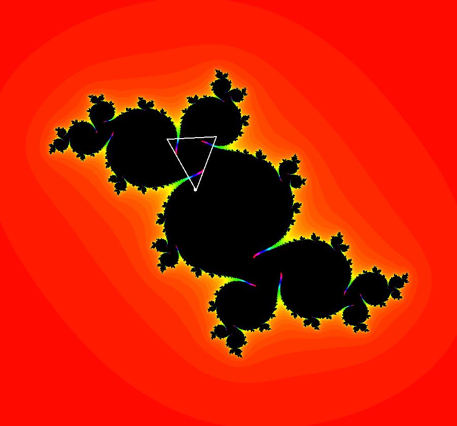
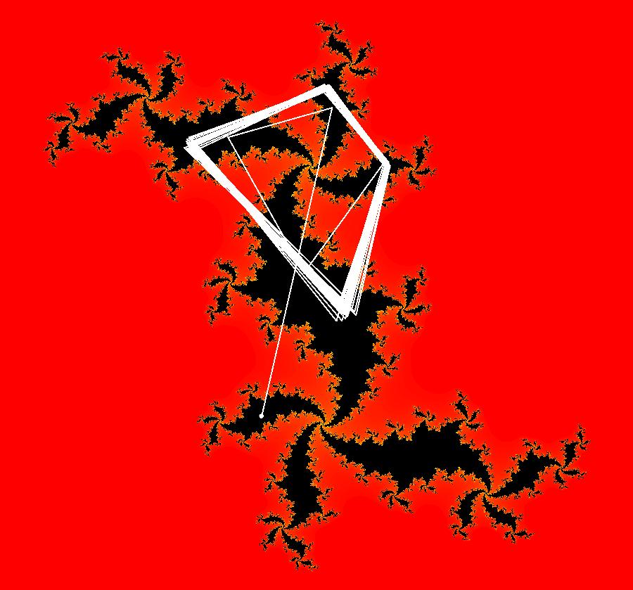
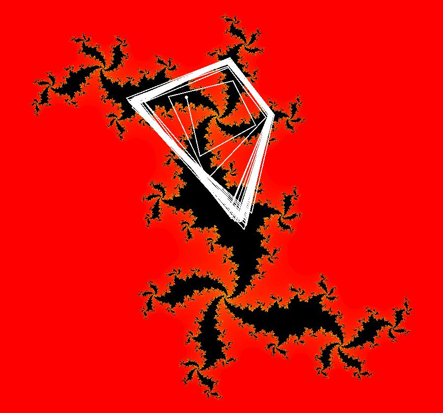
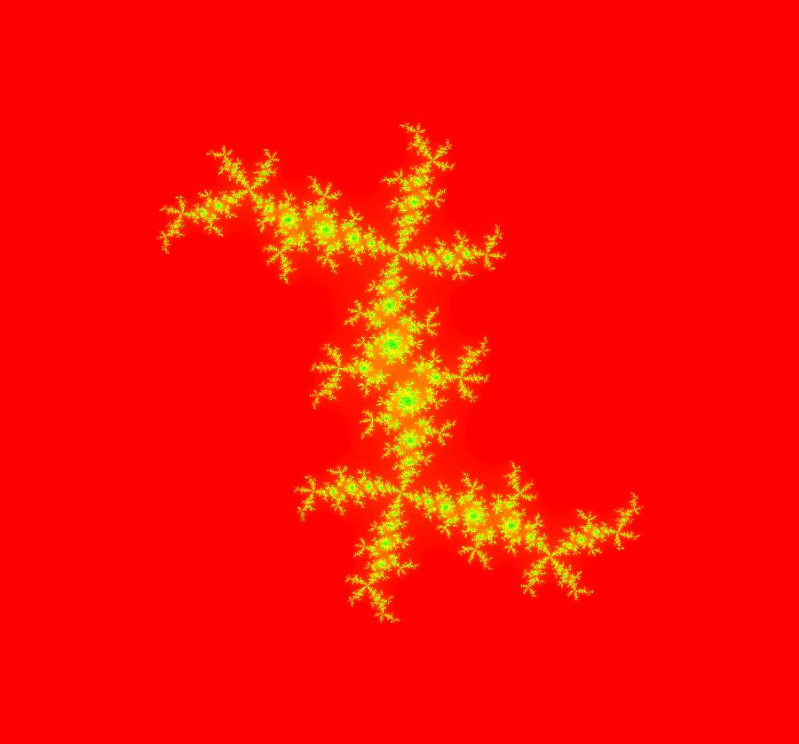
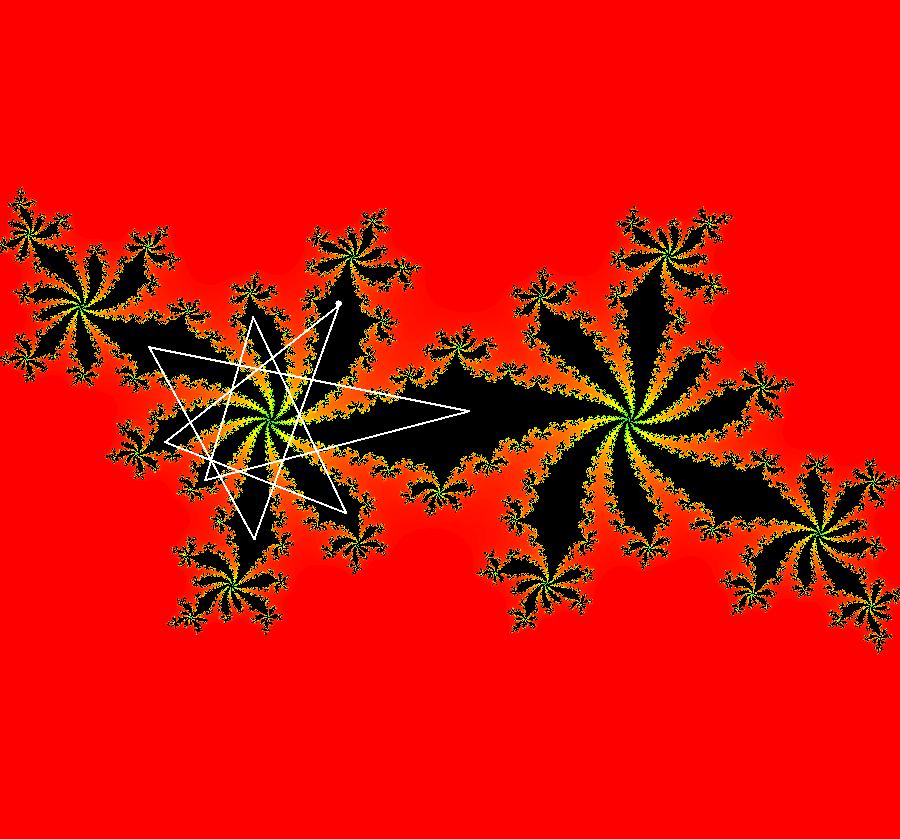
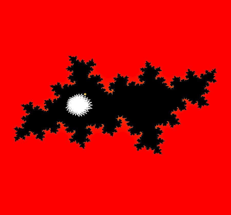
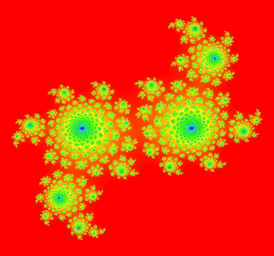
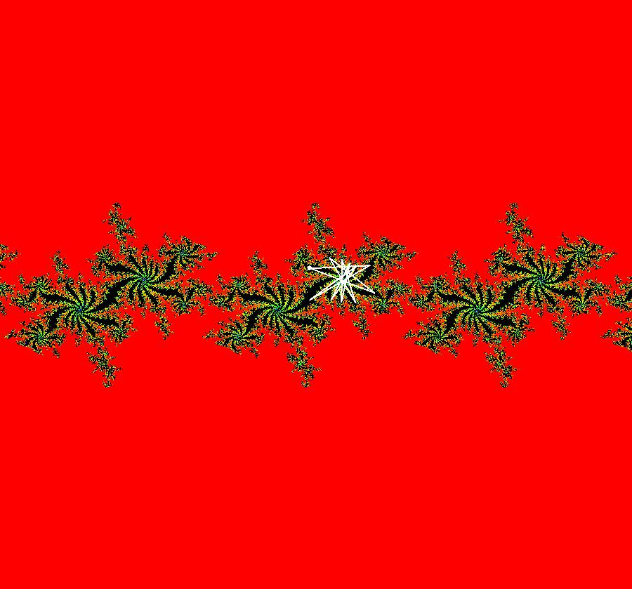
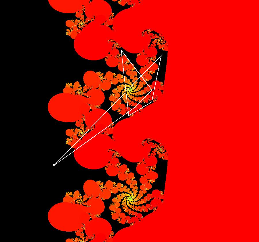
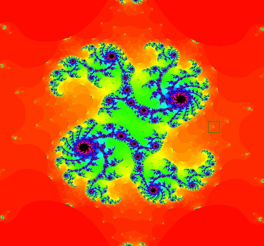
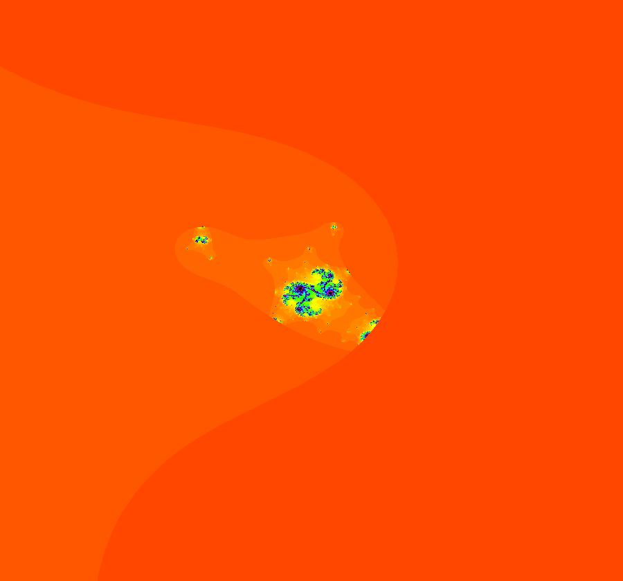
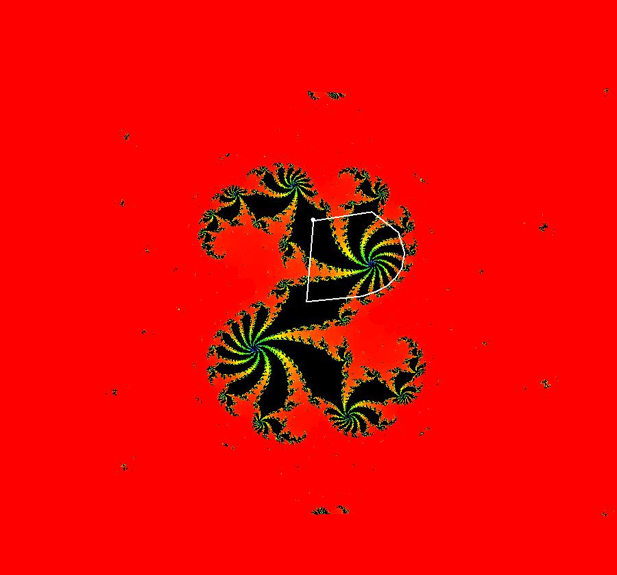
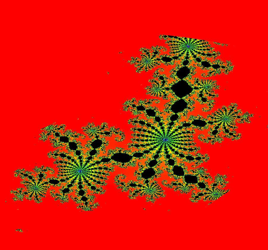
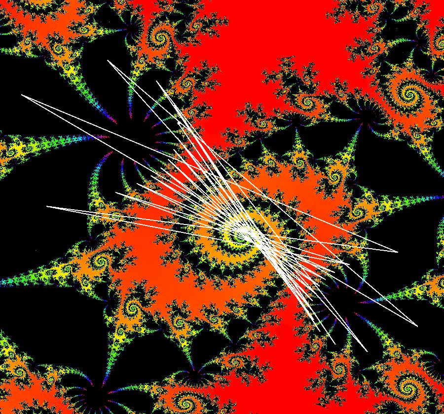
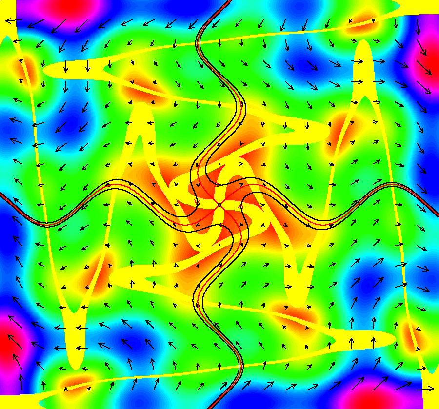
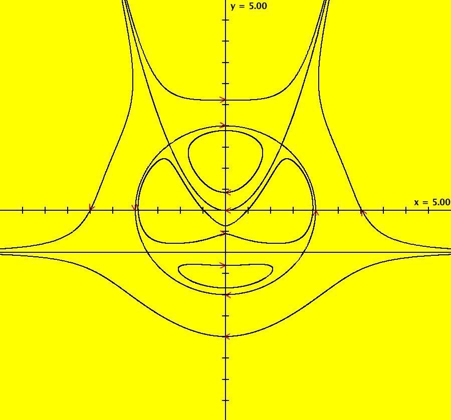
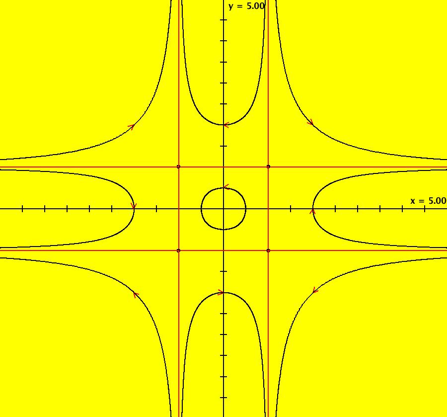
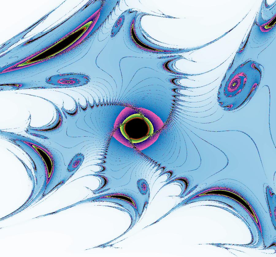
View/Sys/Gal: EMap "AGFExs: deg 3-: (1) AGF star in & star out" in "VectorFields." The next 8 systems are based on this "star in & star out" image, which is similar to the image at the top of the OdeFactory User Guide. The image is an example of an AGF. The generators are two symmetric complex lines. Local topological features such as, fixed points and separatrices, have long been used to classify 2D systems of odes. In 1973 I began investigating the idea of using the topological features themselves to generate, or synthesize, odes (vector fields). This lead to my work on "AGFs." The idea is similar to using the conservation of energy (Hamiltonian functions) to generate the equations of motion of mechanical systems. The "star in & star out" AGF system, when written in the traditional "dx/dt, dy/dt" form, is an instance of a Mandelbrot iteration (1980), z<-z^2+c, where z and c are complex. The "star in & star out" AGF system, in "dx/dt, dy/dt" form, when viewed as an iterative system, has the Mandelbrot set as its bifurcation diagram. See systems "deg 3-:" (5) through (8). The AGF is generated by the lines: I[1]: (x+1)+i*y = 0, λ1 = -2, I[2]: (x-1)+i*y = 0, λ2 = 2. The degree of the RHS of an AGF generated by 2 complex lines is, in general 3, but because this system has a symmetric vector field:
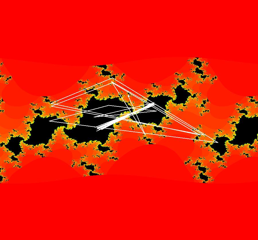
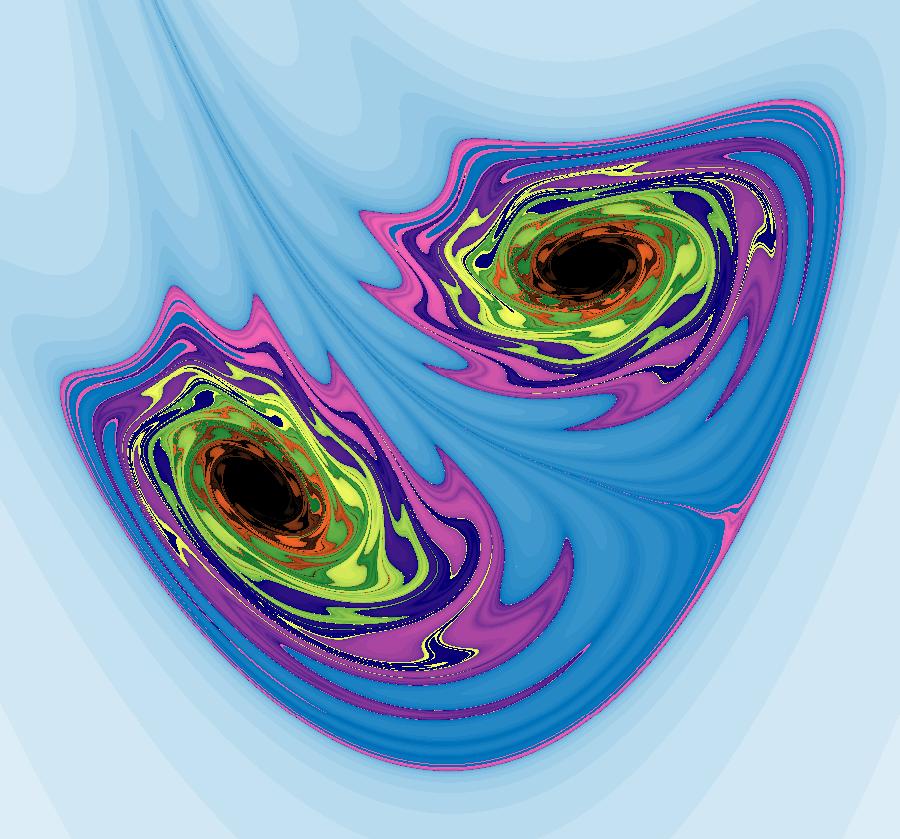
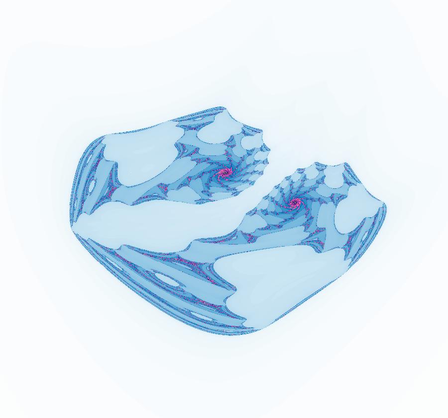
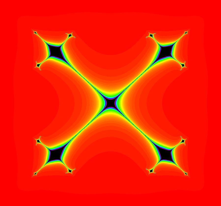
V(-x,-y) = V(x,y), the degree reduces to 2, hence the "deg 3-" name. To verify that the degree of the system is 2, you can use "Insert Equations" to see the expanded "dx/dt, dy/dt" form of the system in the dx/dt and dy/dt fields: dx/dt = ((-1.000*(x+1.000))*((0.500*(x-1.000)^2)+(0.500*(y)^2))+(1.000*(x-1.000))*((0.500*(x+1.000)^2)+(0.500*(y)^2))), dy/dt = -(((1.000*(y))*((0.500*(x-1.000)^2)+(0.500*(y)^2))+(-1.000*(y))*((0.500*(x+1.000)^2)+(0.500*(y)^2)))). These expressions simplify to: dx/dt = x^2-y^2+p, p = -1, dy/dt = 2*x*y+q, q = 0 which gives a classic Mandelbrot/Julia set in the EMap view. Image 1: Ode view of the AGF system. Image 2: EMap Julia set view of the AGF system zoomed in 1X.
|
|
|
View/Sys/Gal: EMap "AGFExs: deg 3-: (2) dx/dt, dy/dt form of star in & star out" in "VectorFields." This system of odes is defined by the equations: dx/dt = x^2-y^2+p, dy/dt = 2*x*y+q. Parameters are: p=-1; q=0 Image 1: Ode view. Image 2: EMap view. Clicking the 4D0P button gives the companion 4D0P system: dx/dt = x, dy/dt = y, dz/dt = z^2-w^2+x, dw/dt = 2*z*w+y.
|
|
|
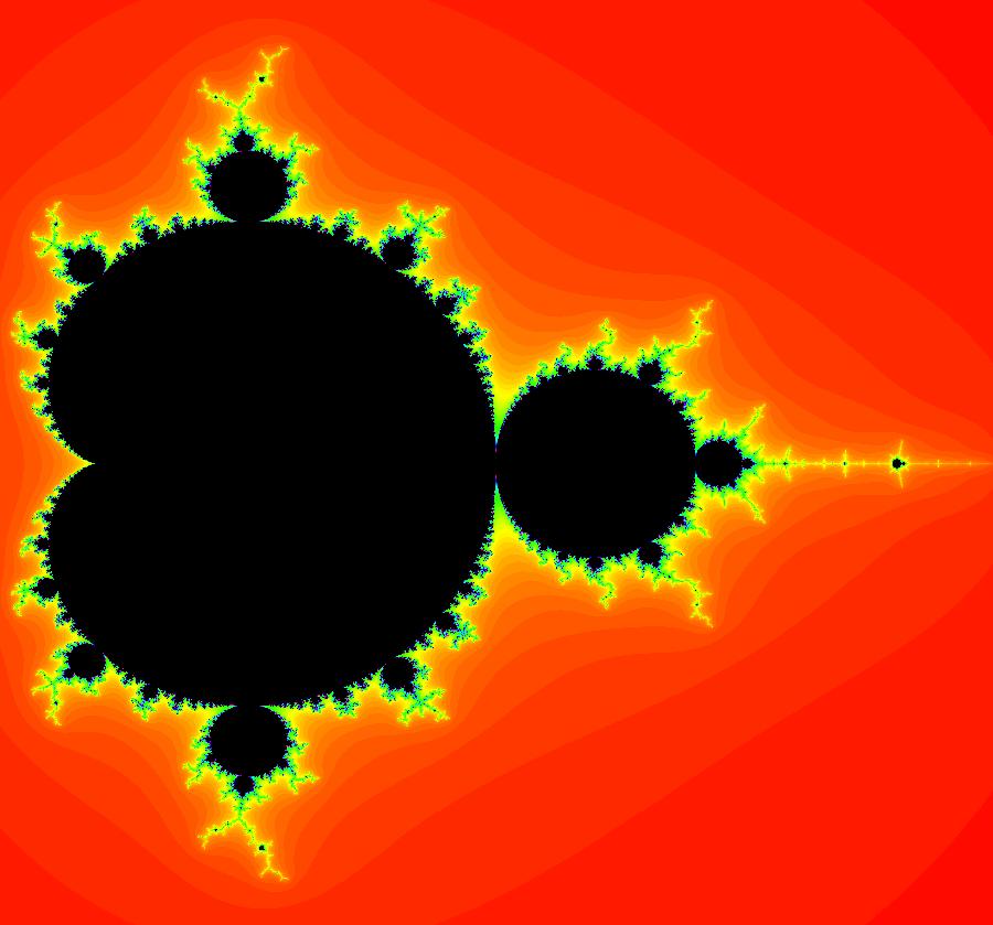
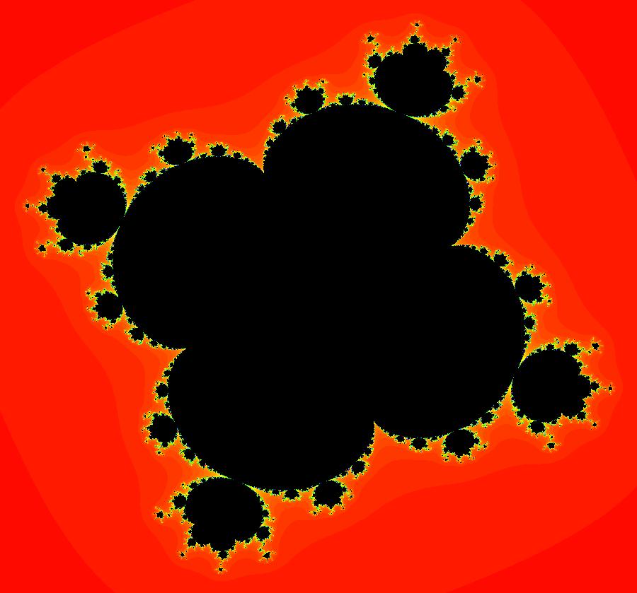
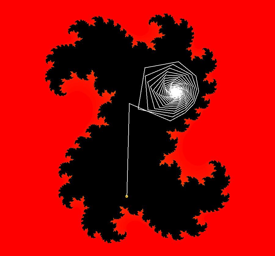
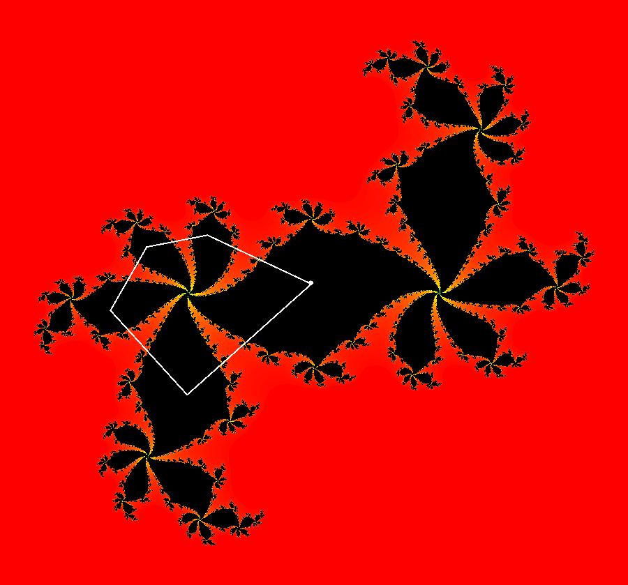
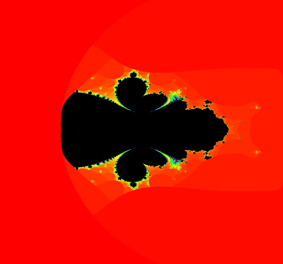
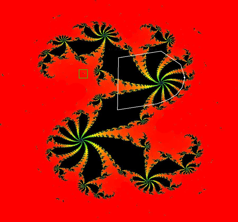
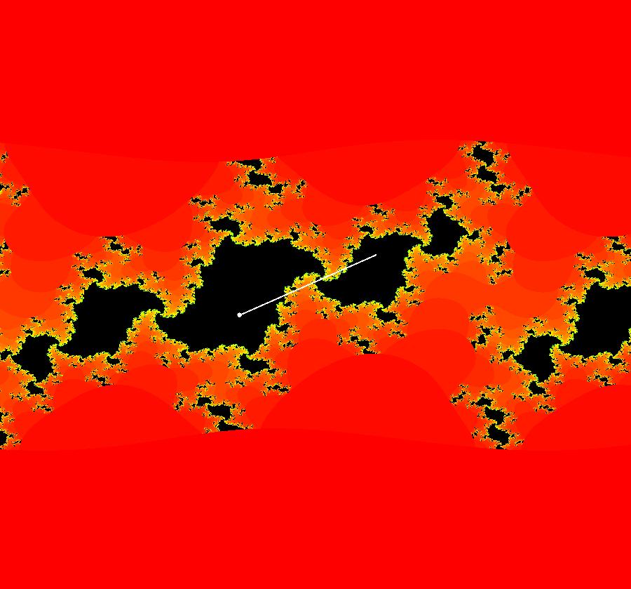
View/Sys/Gal: EMap "AGFExs: deg 3-: (3) Mandelbrot set, EMap view" in "VectorFields." This system of iterations is defined by: x <- x, y <- y, z <- z^2-w^2+x, w <- 2*z*w+y. It is the 4D0P companion to the previous 2D2P system: x <- x^2-y^2+p, y <- 2*x*y+q. The "x" and "y" in the 4D0P system are the "p" and "q" in the 2D system and the "z" and "w" in the 4D0P system are the "x" and "y" in the 2D2P system. Image 1: The (x,y) EMap view of the 4D0P system. This is the Mandelbrot set.
|
|
|
View/Sys/Gal: EMap "AGFExs: deg 3-: (4) AGF perpendicular to star out, star in" in "VectorFields." This AGF is generated by the lines: I[1]: (x+1)+i*y = 0, λ1 = i I[2]: (x-1)+i*y = 0, λ2 = -i The degree of the RHS of the system is 2 due to symmetry. The AGF is: dx/dt = -x*y, dy/dt = -0.5(1-x^2+y^2), As AGFs, (1) and (4) differ only in the eigenvalues. In (1) they are real and in (4) they are complex. Image 1: Ode view. Image 2: EMap view.
|
|
|
View/Sys/Gal: EMap "AGFExs: deg 3-: (5) dx/dt, dy/dt form of (4)" in "VectorFields." This system of odes is defined by the equations: dx/dt = -x*y, dy/dt = -0.5*(1-x^2+y^2). Image 1: Ode view. Image 2: EMap view.
|
|
|
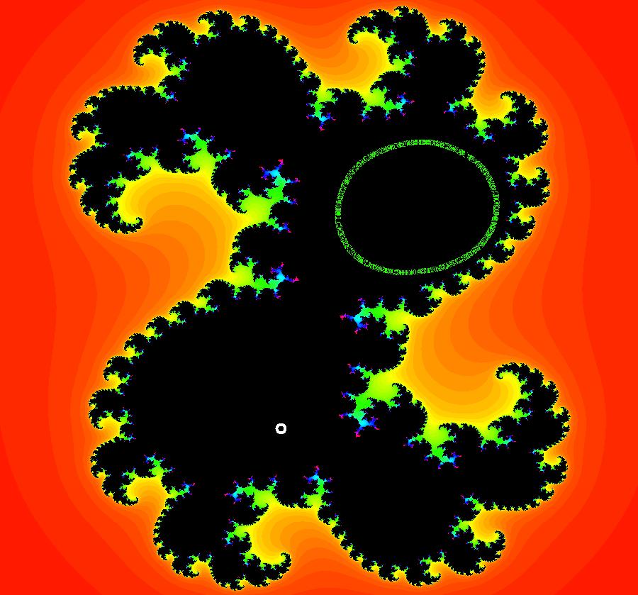
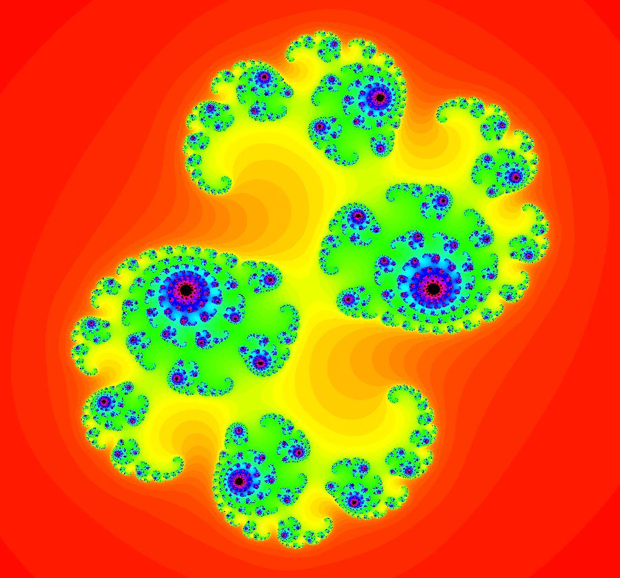
View/Sys/Gal: Ode "AGFExs: deg 3-: (6) EMap (-x*y+p,-0.5*(1-x^2+y^2)+q), p = 1.300; q = 1.100; " in "VectorFields." This iteration is defined by: x <- -x*y+p, y <- -0.5*(1-x^2+y^2)+q. Parameters are: p = 1.300; q = 1.100; EMap CT: 0 A Julia set of system (5) when p and q are added. Image 1: EMap view. Image 2: Ode view.
|
|
|
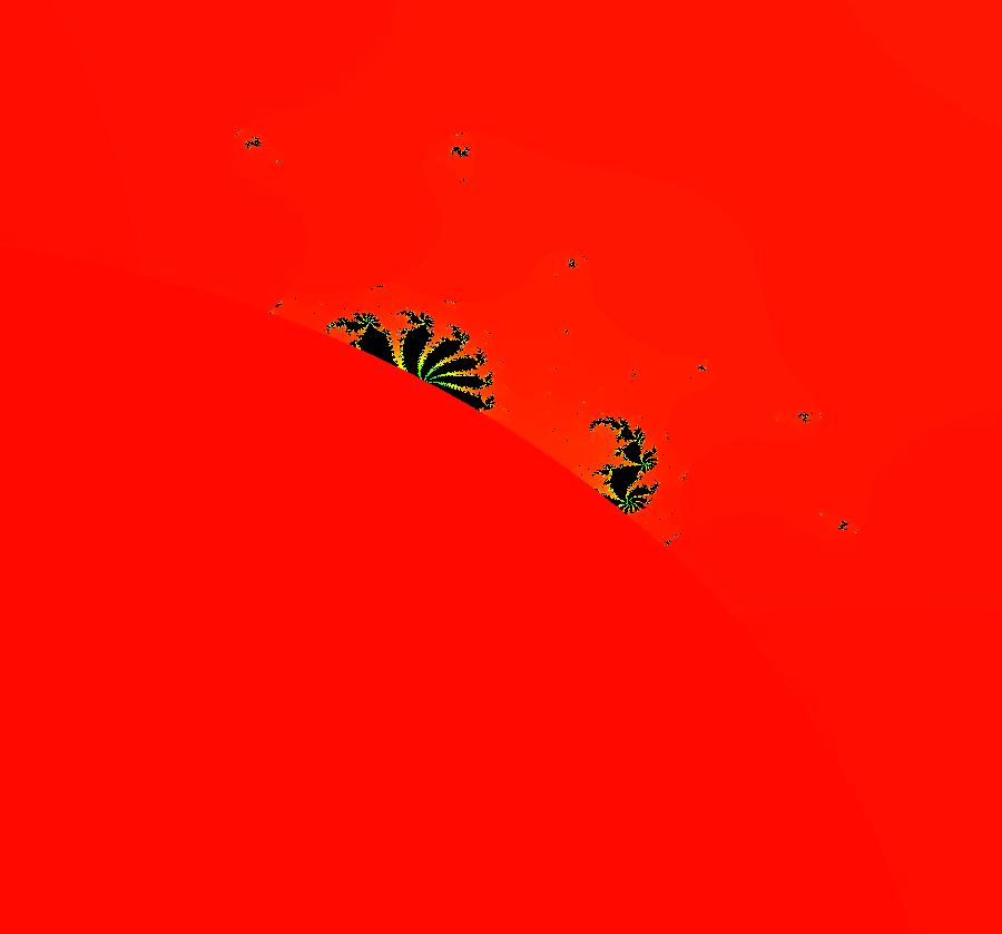
View/Sys/Gal: EMap "AGFExs: deg 3-: (7) (x,y,-z*w+x,-0.5*(1-z^2+w^2)+y) EMap" in "VectorFields." This system of odes is defined by the equations: dx/dt = x, dy/dt = y, dz/dt = -z*w+x, dw/dt = -0.5*(1-z^2+w^2)+y. Mandelbrot set rotated cw 90 degrees. Image 1: EMap view.
|
|
|
View/Sys/Gal: EMap "AGFExs: deg 3-: (8) EMap rotated Mandelbrot set from star in, star out AGF" in "VectorFields." This system of odes is defined by the equations: dx/dt = x, dy/dt = y, dz/dt = 0.5*(1-z^2+w^2)+x, dw/dt = -z*w+y. Mandelbrot set rotated cw 180 degrees. Image 1: EMap view.
|
|
|
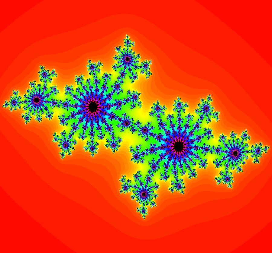
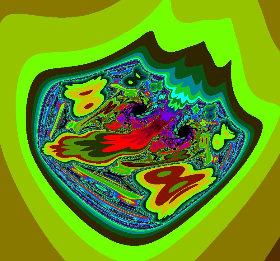
View/Sys/Gal: EMap "AGFExs: deg 3-: (9) nice EMapCT6 (x,y,0.5*(1-z^2+w^2)+x,-z*w+y)" in "VectorFields." This system of odes is defined by the equations: dx/dt = x, dy/dt = y, dz/dt = 0.5*(1-z^2+w^2)+x, dw/dt = -z*w+y. A zoomed in "Art" view of part of the Mandelbrot set using CT6. Image 1: EMapCT6 view.
|
|
|
View/Sys/Gal: Ode "AGFExs: deg 3: 2 complex lines" in "VectorFields." This AGF is generated by the lines: I[1]: x+i*(y-0.5) = 0, λ1 = (1+i) I[2]: x+i*(y+0.48) = 0, λ2 = (-1+i) The degree of the RHS of the system is: 3. Image 1: Ode view.
|
|
|
View/Sys/Gal: EMap "AGFExs: deg 3: 2 complex lines, EMap ver2" in "VectorFields." This AGF is generated by the lines: I[1]: x+i*(y-0.5) = 0, λ1 = (1+i) I[2]: (1+0.01*i)*(x-0.01)+(-0.01+i)*(y+0.46) = 0, λ2 = (-1.3+1.8*i) The degree of the RHS of the system is: 3. Image 1: This EMap was arrived at by adjusting the control parameters for I[2] in the previous system.
|
|
|
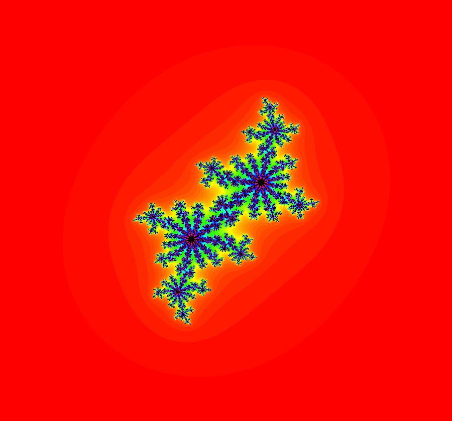
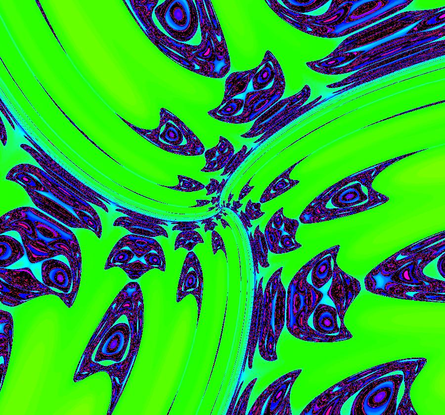
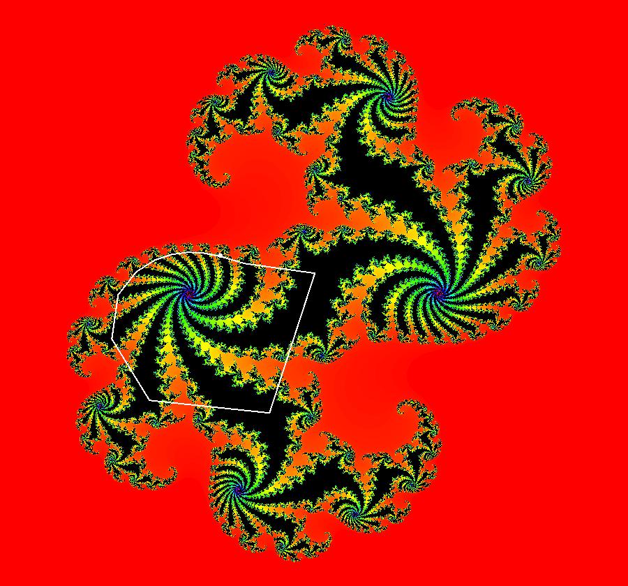
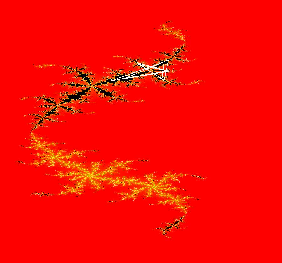
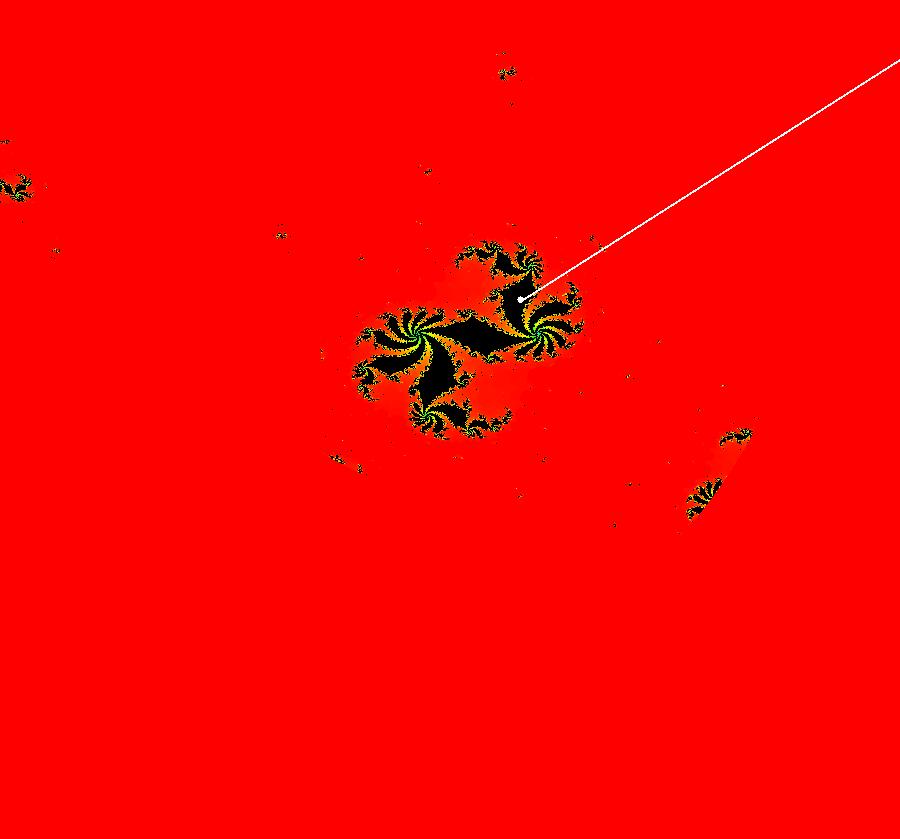
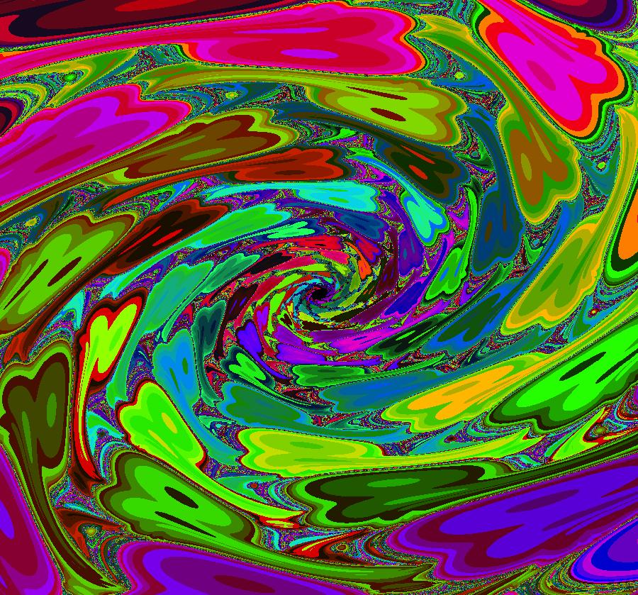
View/Sys/Gal: EMap "AGFExs: deg 3: 2 complex lines, EMap ver3, JavaCats" in "VectorFields." This AGF is generated by the lines: I[1]: x+i*(y-0.5) = 0, λ1 = (1+i) I[2]: (1+0.01*i)*(x-0.01)+(-0.01+i)*(y+0.46) = 0, λ2 = (-1.3+1.8*i) The degree of the RHS of the system is: 3. Image 1: EMap view of the previous system zoomed in at the fractal center (-.3965347,.1744894).
|
|
|
View/Sys/Gal: EMap "AGFExs: deg 3: 2 complex lines, EMapCT1 ver1" in "VectorFields." This AGF is generated by the lines: I[1]: (0.4+0.29*i)*(x+0.2)+(-0.49+i)*(y-0.44) = 0, λ1 = (4.4+1.2*i) I[2]: x+i*(y+0.48) = 0, λ2 = (-1+i) The degree of the RHS of the system is: 3. This EMap was arrived at by adjusting the I[1] parameters. Image 1: EMapCT1 view. This is a fractal but not a fractal center.
|
|
|
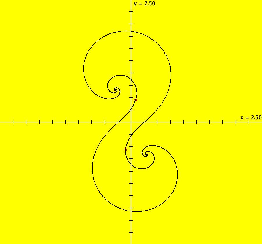
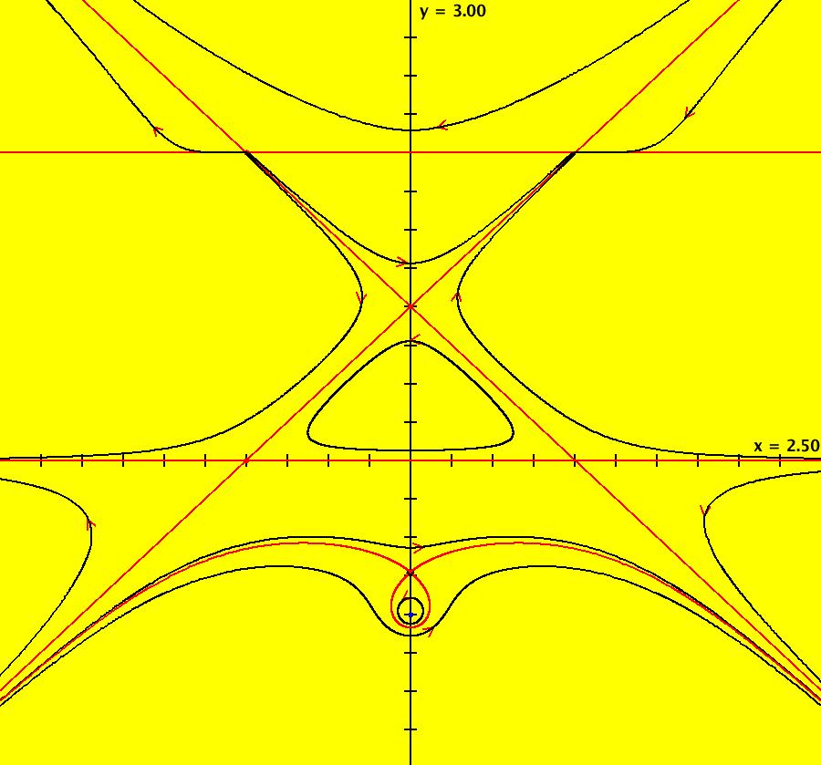
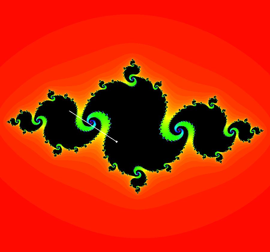
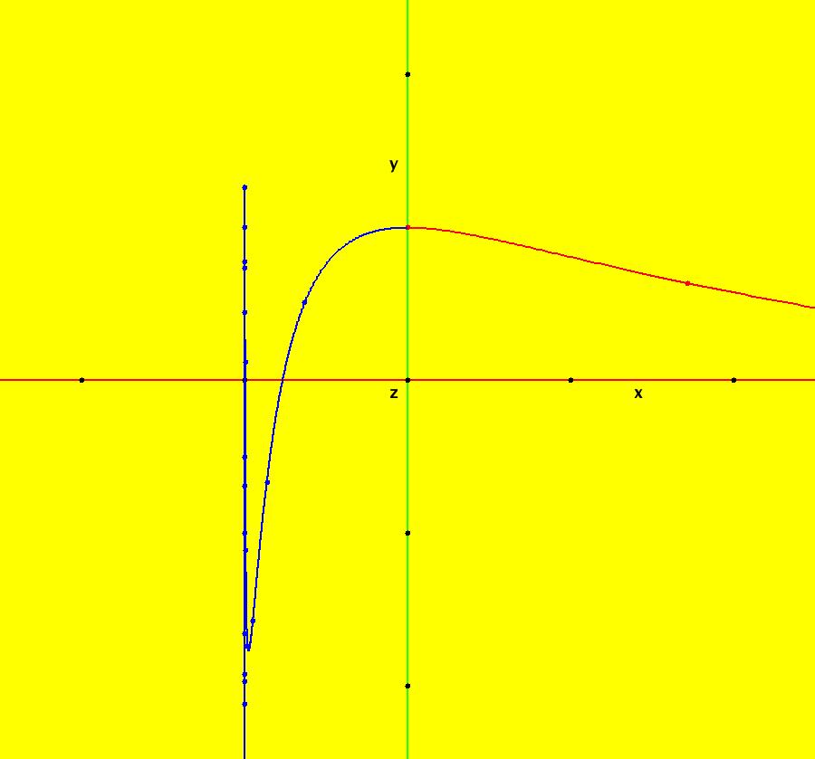
View/Sys/Gal: Ode "AGFExs: deg 3: limit flow, fig 3.3 of AGF book" in "VectorFields." This system of odes is defined by the equations: dx/dt = -(k*y-a/2)*P-a*y^2, dy/dt = x*(k*P+a*y). Parameters are: k = 1; a = 2 Functions are: P = x^2+y^2-1 Image 1: Ode view.
|
|
|
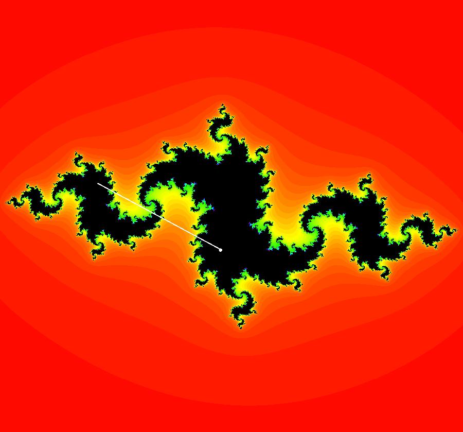
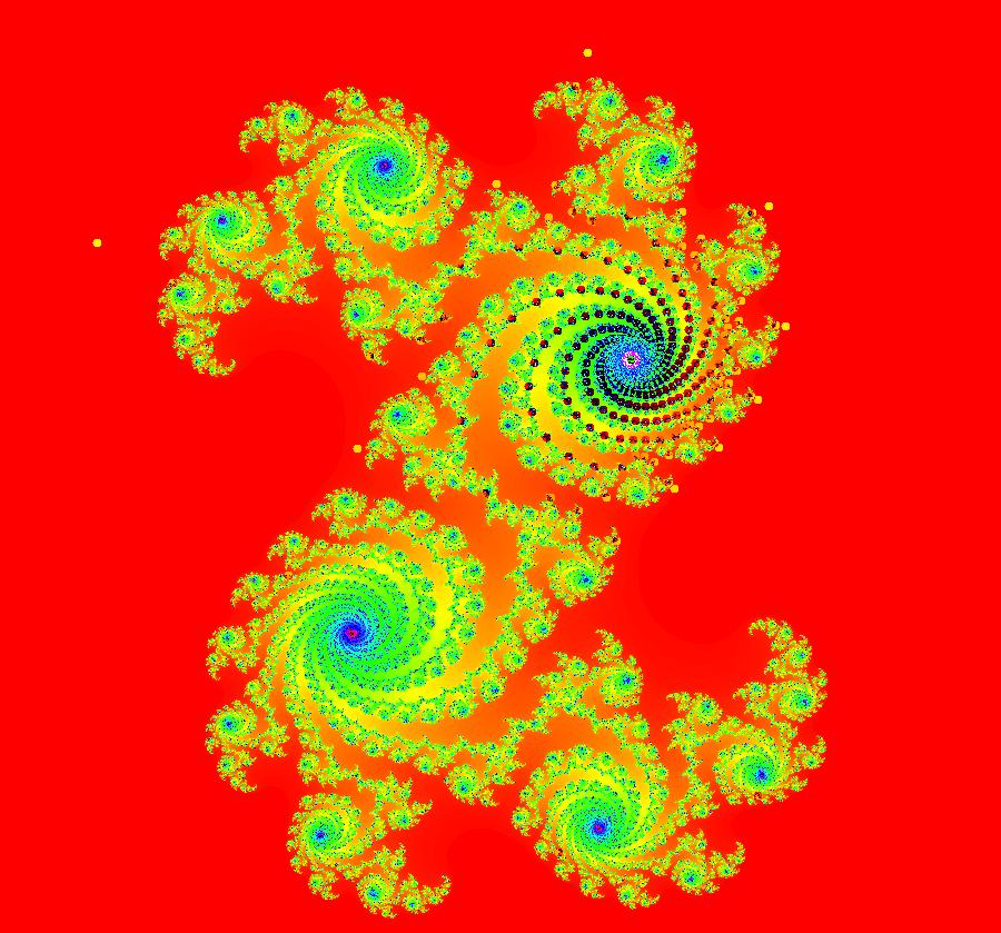
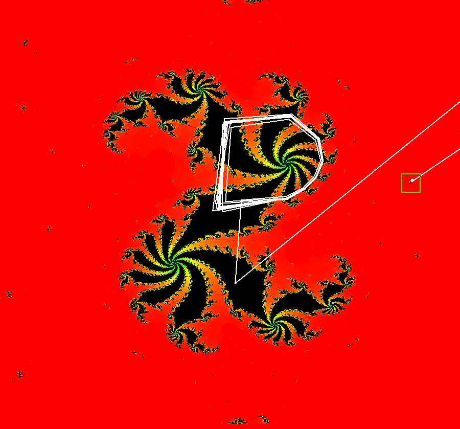
View/Sys/Gal: EMap "AGFExs: deg 3: limit flow, fig 3.3 of AGF book, EMap" in "VectorFields." This iteration is defined by: x <- -(k*y-a/2)*P-a*y^2, y <- x*(k*P+a*y). Parameters are: k = .50; a= 1.80; Functions are: P = x^2+y^2-1 Image 1: EMap view. This is a fractal. Try adjusting the parameters.
|
|
|
View/Sys/Gal: EMap "AGFExs: deg 3: limit flow, fig 3.3 time-scaled, EMapCT3" in "VectorFields." This iteration is defined by: x <- (1+s*.01)*(-(k*y-a/2)*P-a*y^2), y <- (1+s*.01)*x*(k*P+a*y). Parameters are: k = .48; a = 1.80; s = 5.70; Functions are: P = x^2+y^2-1 Image 1: EMapCT3 view. Zoom in to see the fractal nature of this EMap. The time-scaling factor, (1+s*.01), gives finer control over the size of the black regions called basins of attraction.
|
|
|
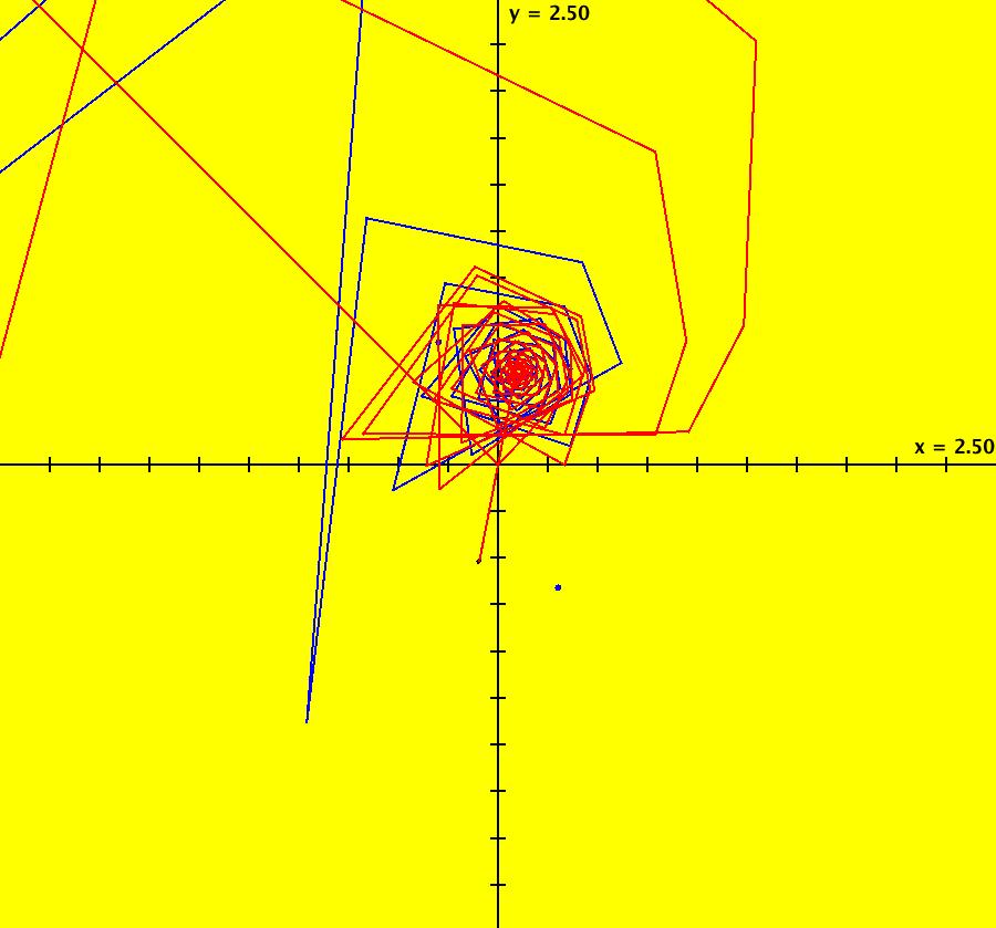
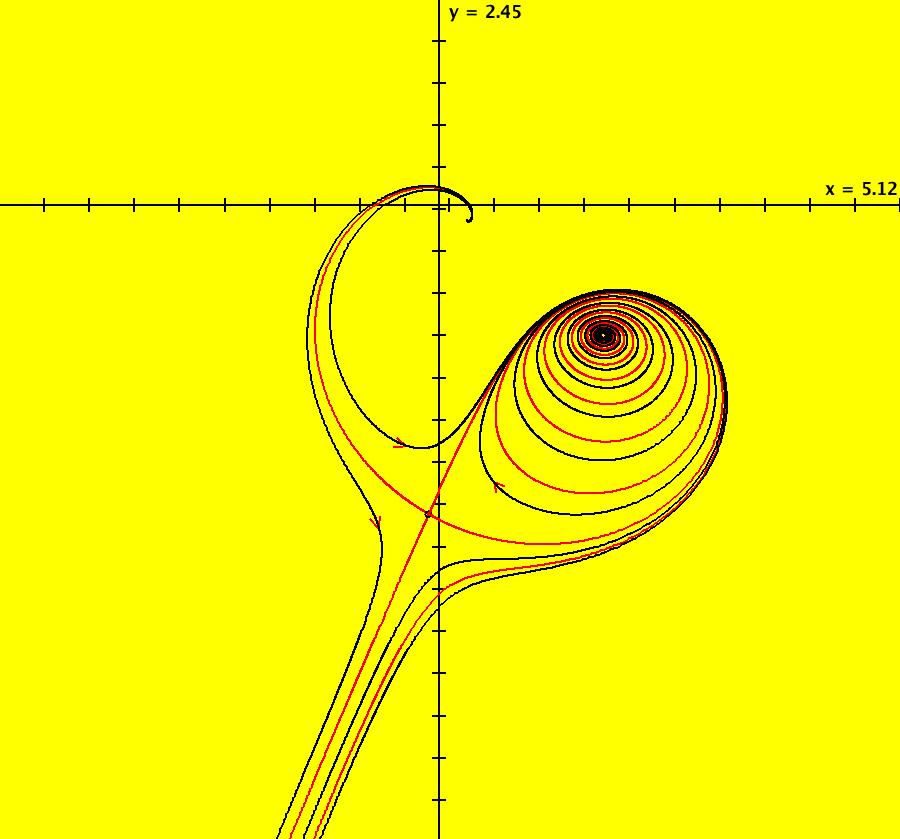
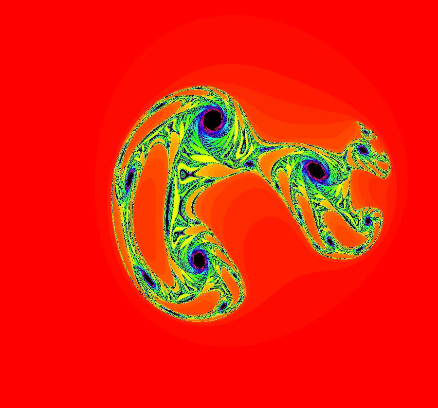
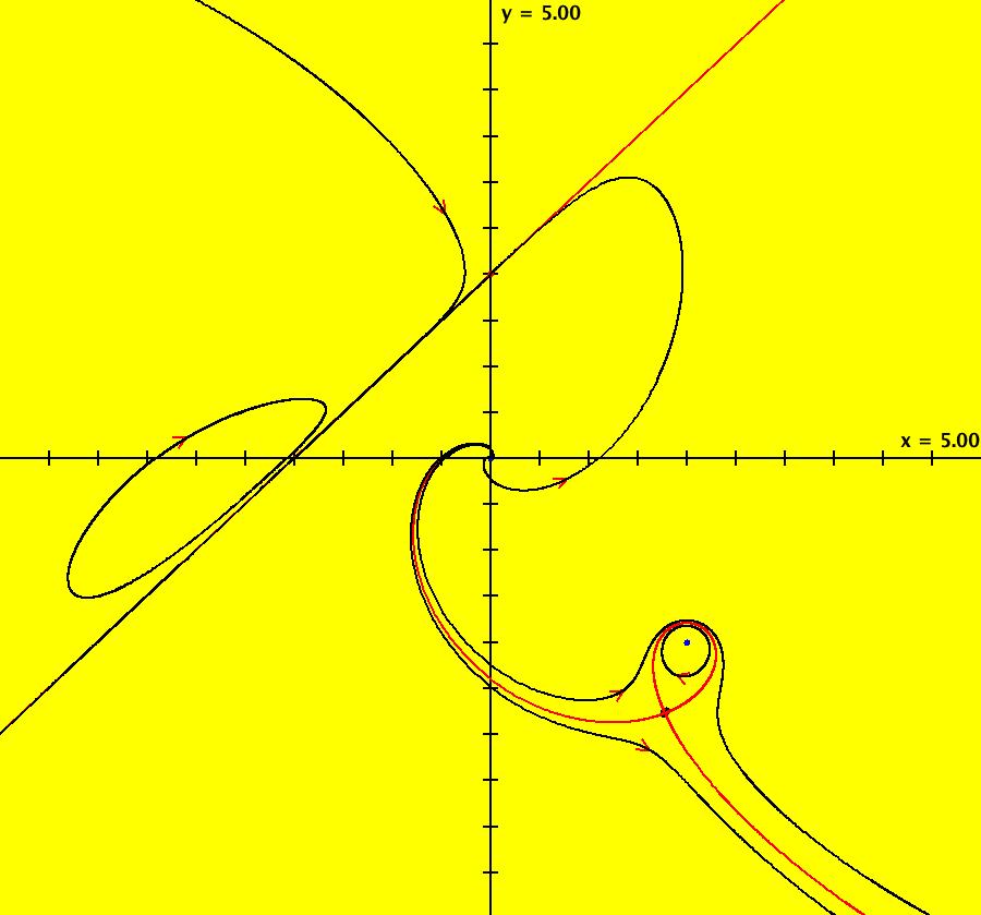
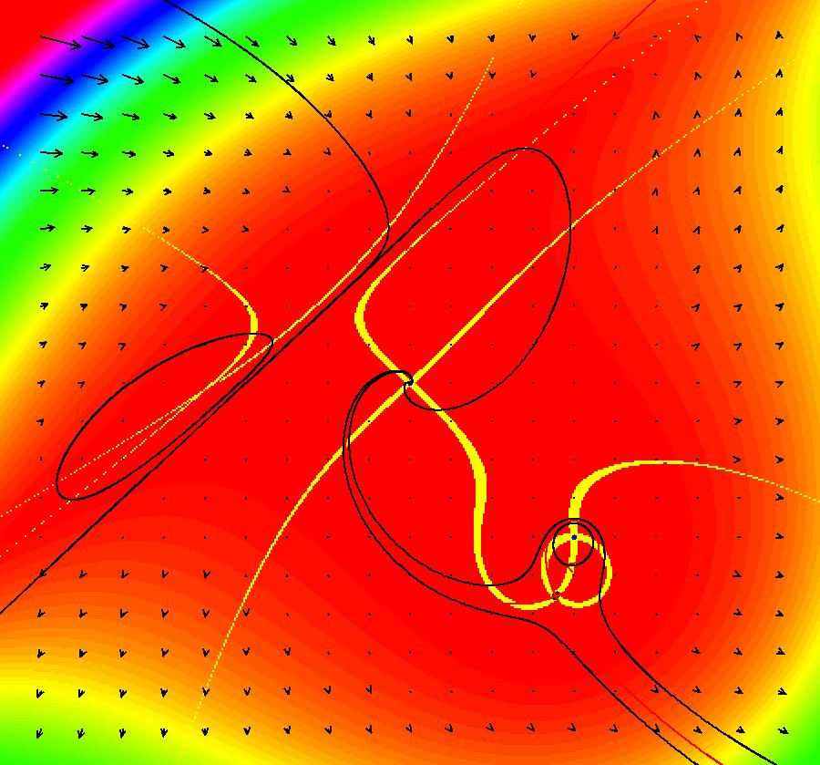
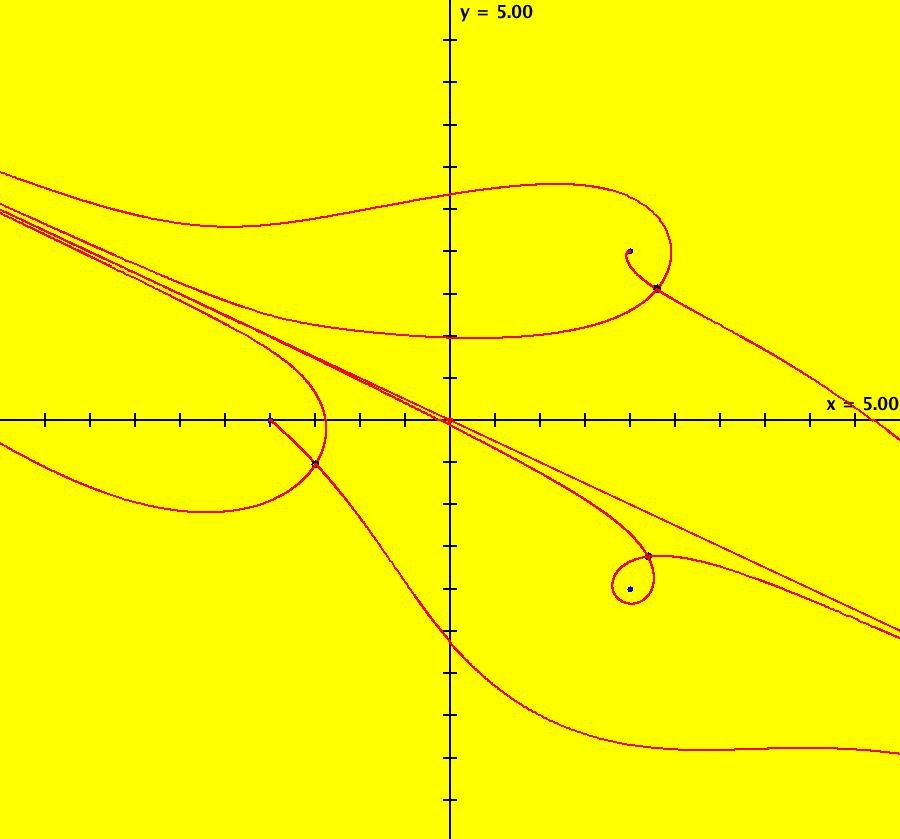
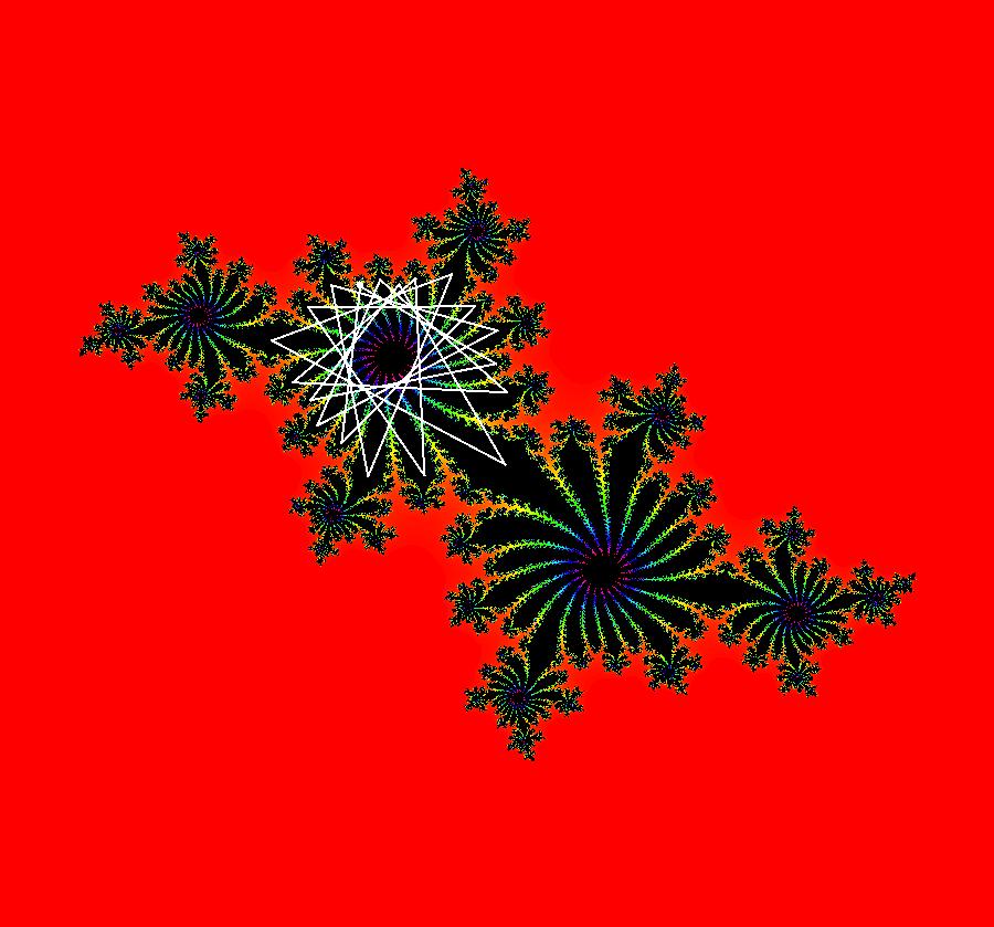
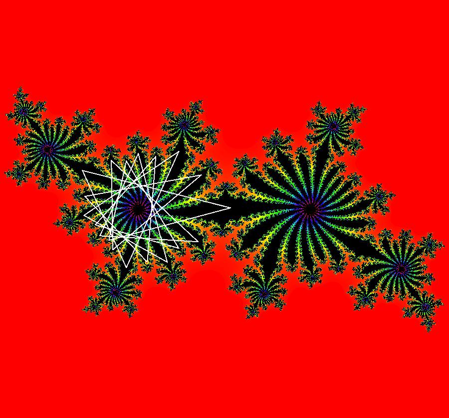
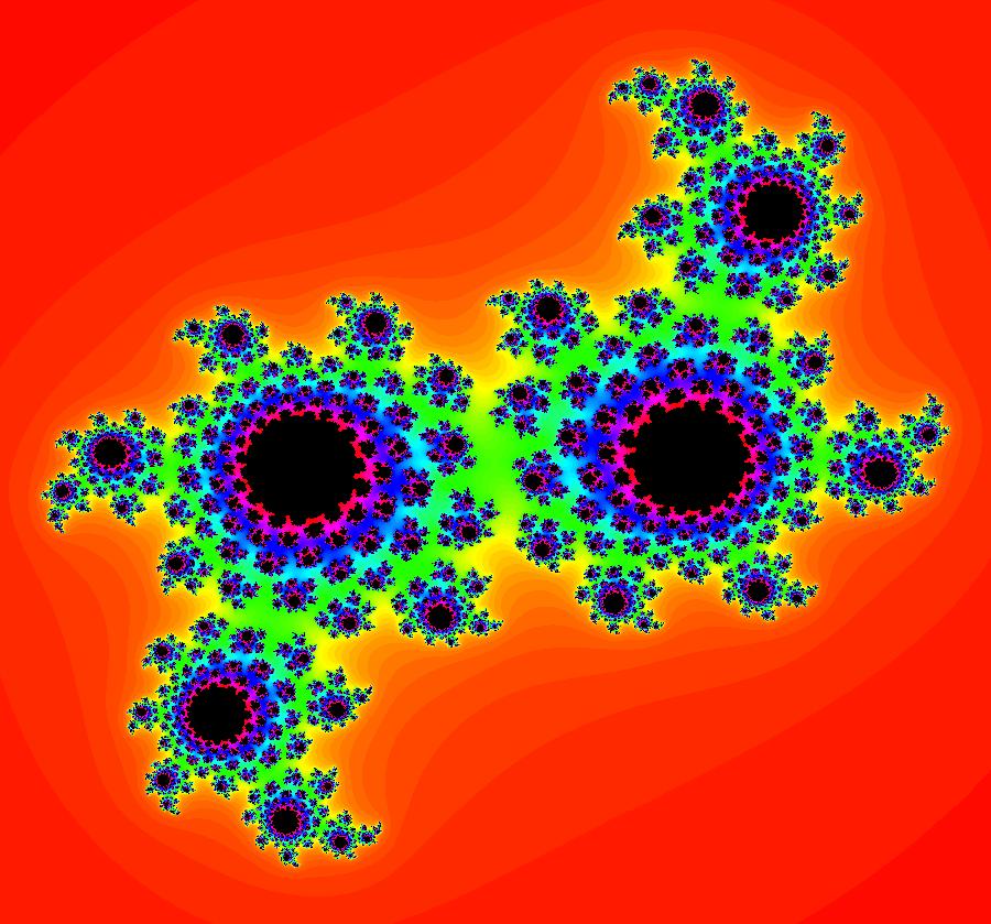
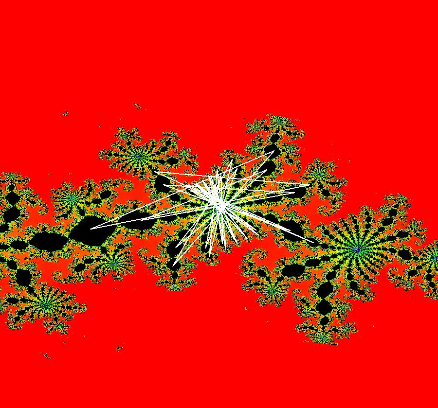
View/Sys/Gal: EMap "AGFExs: deg 3: spiral out and center" in "VectorFields." This AGF is generated by the lines: I[1]: (x-2)+i*(y+2) = 0, λ1 = i, center I[2]: x+i*y = 0, λ2 = (1-i), spiral out The degree of the RHS of the system is: 3. Or: dx/dt = 0.125*(x^3-2*x^2+x*(y^2+8*y+8)-2*y*(y+4)), dy/dt = 0.125*(x^2*(y-2)+8*x+y*(y^2+6*y+8)). Image 1: Ode view. This has several fractal centers. Image 2: EMapCT5 view.
|
|
|
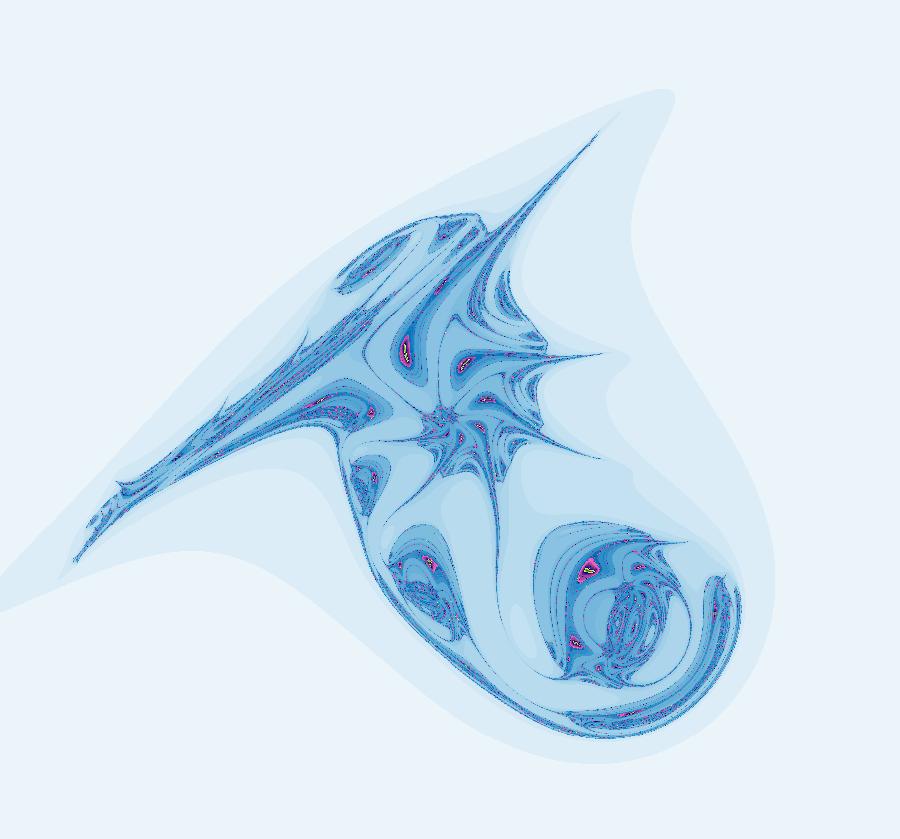
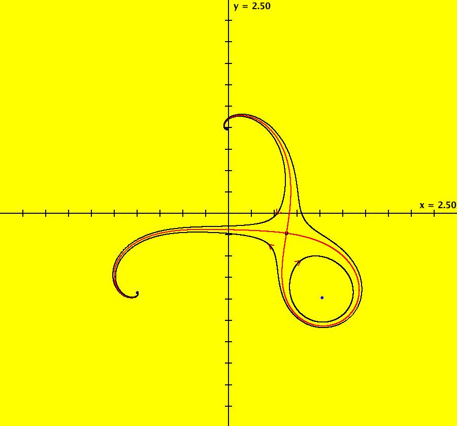
View/Sys/Gal: EMap "AGFExs: deg 3: spiral out and center, dx/dt, dy/dt form, ver2" in "VectorFields." This system of odes is defined by the equations: dx/dt = 0.125*(x^3-2*x^2+x*(y^2+8*y+8)-2*y*(y+4))+p dy/dt = 0.125*(x^2*(y-2)+8*x+y*(y^2+6*y+8))+q Parameters are: p = -.42; q = -.13; For these parameter values the system becomes spiral out and spiral in. For p = q = 0 we get the previous spiral out and center system. The parameters were added to the system to make the EMaps more interesting. Image 1: Ode view. Image 2: EMap view.
|
|
|
View/Sys/Gal: Ode "AGFExs: deg 4: 3 real lines, 1 complex line, ver1" in "VectorFields." This AGF is generated by the lines: L[1]: (x+1)-y = 0, m1 = 1, λ1 = -1 L[2]: x+(y-1) = 0, m2 = -1, λ2 = -1 L[3]: y = 0, m3 = 0, λ3 = 1 I[1]: x+i*(y-0.5) = 0, λ1 = (1-i) The degree of the RHS of the system is: 4. Image 1: Ode view.
|
|
|
View/Sys/Gal: Ode "AGFExs: deg 4: 3 real lines, 1 complex line, ver2" in "VectorFields." This AGF is generated by the lines: L[1]: (x+1)-y = 0, m1 = 1, λ1 = -1 L[2]: x+(y-1) = 0, m2 = -1, λ2 = -1 L[3]: y = 0, m3 = 0, λ3 = 1 I[1]: (x+0.01)+i*(y+0.99802) = 0, λ1 = (1-i) The degree of the RHS of the system is: 4. Image 1: Ode view.
|
|
|
View/Sys/Gal: Ode "AGFExs: deg 4: 3 real lines, 1 complex line, ver3" in "VectorFields." This AGF is generated by the lines: L[1]: (x+1)-y = 0, m1 = 1, λ1 = -1 L[2]: x+(y-1) = 0, m2 = -1, λ2 = -1 L[3]: y = 0, m3 = 0, λ3 = 1 I[1]: x+i*(y+1) = 0, λ1 = -i The degree of the RHS of the system is: 4. Image 1: Ode view.
|
|
|
View/Sys/Gal: Ode "AGFExs: deg 4: 5 real lines" in "VectorFields." This AGF is generated by the lines: L[1]: (x+1)-y = 0, m1 = 1, λ1 = -1 L[2]: x+(y-1) = 0, m2 = -1, λ2 = -1 L[3]: y = 0, m3 = 0, λ3 = 1 L[4]: (y-2) = 0, m4 = 0, λ4 = 1 L[5]: (y+1) = 0, m5 = 0, λ5 = 1 The degree of the RHS of the system is: 4. Image 1: Ode view.
|
|
|
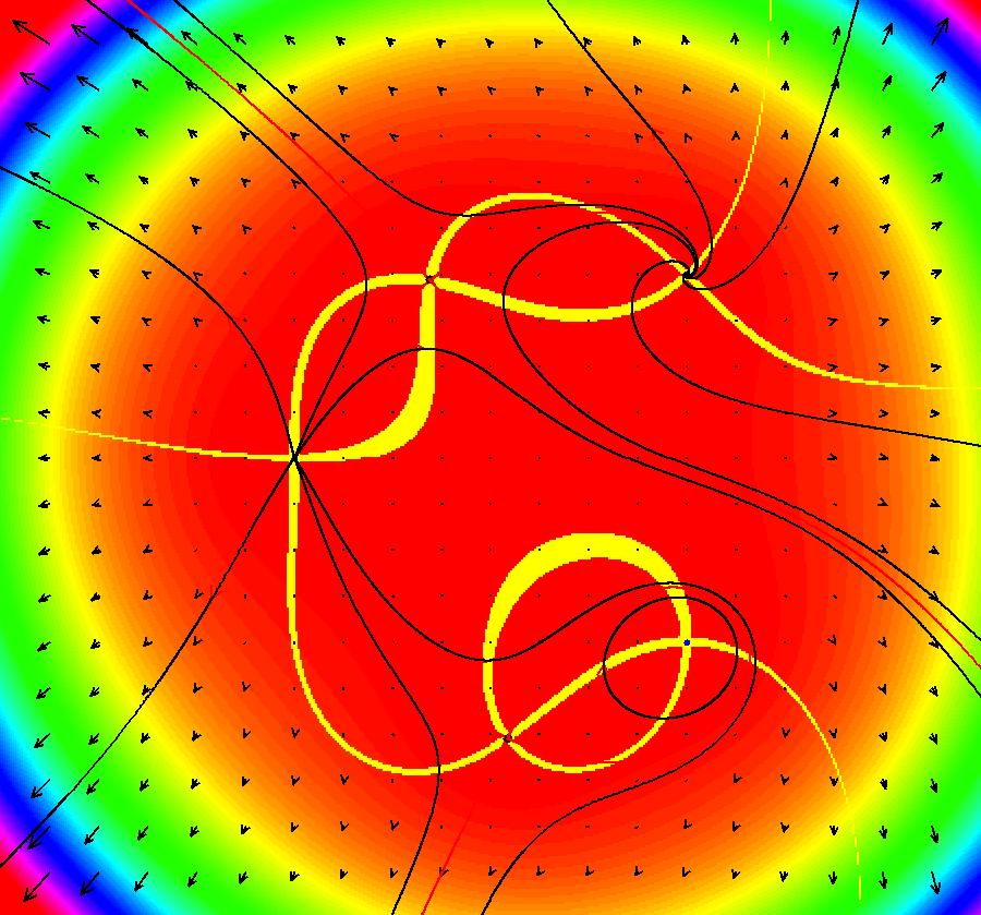
View/Sys/Gal: EMap "AGFExs: deg 4: line, center and spiral out" in "VectorFields." This AGF is generated by the lines: L[1]: x-(y-2) = 0, m1 = 1, λ1 = 1 I[1]: (x-2)+i*(y+2) = 0, λ1 = i I[2]: x+i*y = 0, λ2 = (1-i) The degree of the RHS of the system is: 4. Image 1: Ode view. To see the nullclines, select "Show Colored Vector Field w/Nullclines" on the Help menu than click the "V On" button. Image 2: Nullclines. The EMapCT3 is also worth looking at. Image 3: EMapCT3.
|
|
|
View/Sys/Gal: Ode "AGFExs: deg 5: 3 complex lines" in "VectorFields." This AGF is generated by the lines: I[1]: (x-1.02)+i*(y+0.98814) = 0, λ1 = i I[2]: (x+0.02)+i*(y-0.98814) = 0, λ2 = (1+i) I[3]: (x+1)+i*(y+0.92885) = 0, λ3 = (-1-i) The degree of the RHS of the system is: 5. Image 1: Ode view.
|
|
|
View/Sys/Gal: Ode "AGFExs: deg 5: 4 real lines, 1 complex line" in "VectorFields." This AGF is generated by the lines: L[1]: (x+1)-y = 0, m1 = 1, λ1 = -1 L[2]: x+(y-1) = 0, m2 = -1, λ2 = -1 L[3]: y = 0, m3 = 0, λ3 = 1 L[4]: (y-2) = 0, m4 = 0, λ4 = 1 I[1]: x+i*(y+1) = 0, λ1 = -i The degree of the RHS of the system is: 5. Image 1: Ode view.
|
|
|
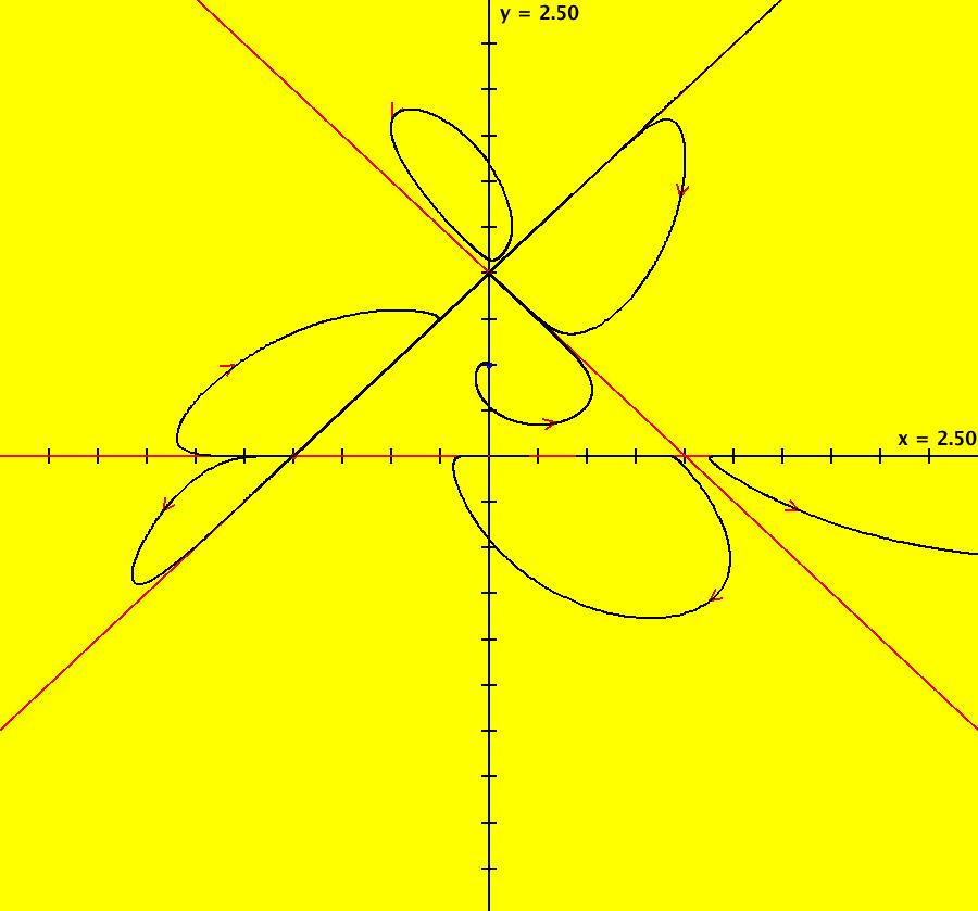
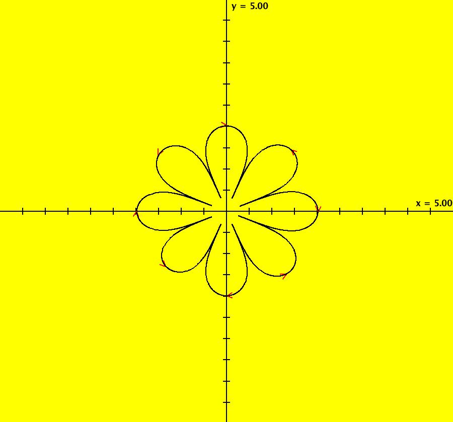
View/Sys/Gal: Ode "AGFExs: deg 5: power flow" in "VectorFields." This system of odes is defined by the equations: dx/dt = y*(5*x^4-10*x^2*y^2+y^4)/4, dy/dt = -x*(x^4-10*x^2*y^2+5*y^4)/4 This is an AGF power flow generated by I = x +i*y with λ = i and power = 5. Critical directions are +-n*pi/8 where n = 1, 3, 9, 11 In general, the class I flow generated by the p-th power of a complex line, where p>1, is a 2*(p-1) leafed flower. Image 1: Ode view.
|
|
|
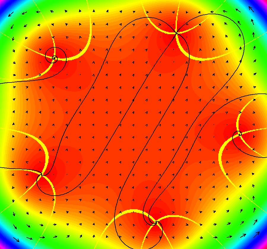
View/Sys/Gal: EMap "AGFExs: deg 5: power flow, w/params, EMap" in "VectorFields." This system of odes is defined by the equations: dx/dt = y*(5*x^4-10*x^2*y^2+y^4)/4+p, dy/dt = -x*(x^4-10*x^2*y^2+5*y^4)/4+q Parameters are: p = .55; q = 1.00; Image 1: Ode view w/colored vector field on. Image 2: EMapCT3 view.
|
|
|
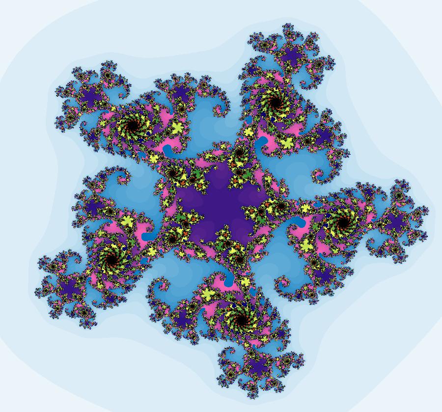
View/Sys/Gal: EMap "AGFExs: deg 5: power flow, w/params, EMap per-3 attractor" in "VectorFields." This iteration is defined by: x <- y*(5*x^4-10*x^2*y^2+y^4)/4+p, y <- -x*(x^4-10*x^2*y^2+5*y^4)/4+q. Parameters are: p = .8277; q = .7371; EMap CT: 0 Image 1: EMap view showing the 3-cycle attractor in the basin of attraction.
|
|
|
View/Sys/Gal: EMap "AGFExs: deg 5: power flow, w/params, EMap, 4D0P companion" in "VectorFields." This system of odes is defined by the equations: dx/dt = x, dy/dt = y, dz/dt = w*(5*z^4-10*z^2*w^2+w^4)/4+x, dw/dt = -z*(z^4-10*z^2*w^2+5*w^4)/4+y. This is a Mandelbrot-like set. It is the 4D0P bifurcation diagram for the previous 2D2P system: dx/dt = y*(5*x^4-10*x^2*y^2+y^4)/4+p, dy/dt = -x*(x^4-10*x^2*y^2+5*y^4)/4+q Image 1: EMap view. The point (p,q) = (.8277,.7371) is in a 3-rd largest lobe. Any point in an n-th largest lobe will give a per-n attractor in the EMap view of the corresponding 2D2P system.
|
|
|
View/Sys/Gal: Ode "AGFExs: deg 5: star out, spiral out, center" in "VectorFields." This AGF is generated by the lines: I[1]: (x+2)+i*y = 0, λ1 = 1 I[2]: (x-2)+i*(y-2) = 0, λ2 = (1-i) I[3]: (x-2)+i*(y+2) = 0, λ3 = i The degree of the RHS of the system is: 5. Image 1: Ode view with nullclines.
|
|
|
View/Sys/Gal: Ode "AGFExs: deg 6: star out, spiral out, center and line" in "VectorFields." This AGF is generated by the lines: L[1]: x+2*y = 0, m = -0.5, λ1 = -1 I[1]: (x+2)+i*y = 0, λ1 = 1 I[2]: (x-2)+i*(y-2) = 0, λ2 = (1-i) I[3]: (x-2)+i*(y+2) = 0, λ3 = i The degree of the RHS of the system is: 6. Image 1: Ode view showing the 4 generators and the separatrix system.
|
|
|
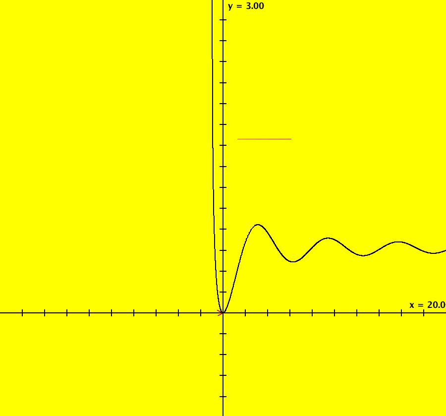
View/Sys/Gal: Ode "AGFExs: deg 7: 4 real lines, 2 complex lines" in "VectorFields." This AGF is generated by the lines: L[1]: (x+1)-y = 0, m1 = 1, λ1 = -1 L[2]: x+(y-1) = 0, m2 = -1, λ2 = -1 L[3]: y = 0, m3 = 0, λ3 = 1 L[4]: (y-2) = 0, m4 = 0, λ4 = 1 I[1]: x+i*(y+1) = 0, λ1 = 20*i I[2]: x+i*(y-0.5) = 0, λ2 = i The degree of the RHS of the system is: 7. Image 1: Ode view.
|
|
An OdeFactory Slide Show Click on a slide to zoom in. Click "video" to see a video. |
View/Sys/Gal: Ode "ComplexFns: ***** Introduction *****" in "VectorFields." ***** Introduction ***** (A) Rewriting z <- f(z,c) as a 2D real system. Given a complex system that is defined using the complex state variable z, and possibly a complex parameter, it is easy to convert the system to the corresponding 2D real system: You can do the conversion by hand or you can enter f(z,c) at z = x+i*y, c = p+i*q into WA (WolframAlpha) then copy/paste the real and complex parts of the result into the x and y OdeFactory entry fields. Note: in the WA conversion you need to insert "*" in the WA expressions for multiplication in OdeFactory. The systems in this gallery are generated as follows. To get system (1) enter the line z^2+c at z = x+i*y, c = p+i*q into WA to get: x <- p+x^2-y^2, y <- q+2*x*y). Systems (2) through (7) are converted in the same way. (B) Finding periodic orbits in 2D fractal images. Systems of the form: z <- f(z,c), c = p+i*q often have EMap images that are fractals. For some particular range of parameter c, a region of the prisoner set can become a basin of attraction. The attractor can be: a fixed point, a limit cycle or a chaotic attractor. It is also possible that there is no attractor. For example every prisoner set orbit of z <- i*z+c, for c = 0, is a different per-4 cycle. Examples in this gallery show how to use OdeFactory to find the basin of attraction, and the attractor(s), for systems of the form: z <- f(z,c), c = p+i*q. Begin by getting into the EMapMax view. Adjust the parameters until you get an image which has a fractal prisoner set where the basic fractal part looks like a flower with petals. Next, with "Show 2D IMap Orbit Sequence" on, start an orbit in a petal and find the end point of the orbit. Start a new orbit at the end point of the orbit and delete the original orbit. The new orbit should be a limit cycle. The period of the limit cycle will equal the number of petals in the flower. If there are two types of petal images, the period is generally the product of the number of petals in the two types of petals. Check additional orbits in the prisoner set to see if each orbit goes to the limit cycle. Different parameter values will result in different fractal images with different limit cycles. For more information regarding Julia sets see Julia Jewels. For more information on chaos see The Chaos Hypertextbook.
|
|
|
View/Sys/Gal: EMap "ComplexFns: EMap 0, z <- i*z+c, c=0+i*0, all per-4" in "VectorFields." This iteration is defined by: x <- y, y <- -x. Parameters are: p=0; q=0 EMap CT: 0 There is a fixed point at (0,0). Except for the fixed point every orbit is a different square. So every orbit in the prisoner set is a different square. There is no prisoner set attractor. Image 1: EMap view. A square per-4 cycle in the prisoner set.
|
|
|
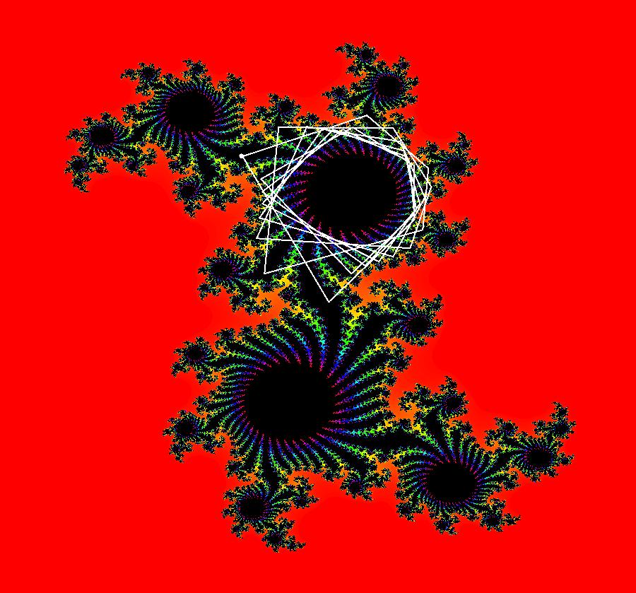
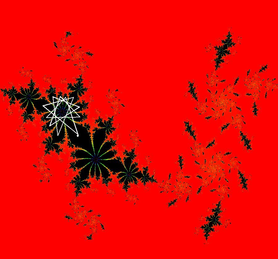
View/Sys/Gal: EMap "ComplexFns: EMap 1a, z <- z^2+c, c=-.06+i*.82, per-3*5" in "VectorFields." This iteration is defined by: x <- p+x^2-y^2, y <- q+2*x*y. Parameters are: p = -.0600; q = .8200; EMap CT: 0 The combination of 3-petals and 5-petals gives a per-15 prisoner set limit cycle attractor. Image 1: EMap view. The per-15 limit cycle.
|
|
|
View/Sys/Gal: EMap "ComplexFns: EMap 1a, z <- z^2+c, c=-.07+i*.68, per-3" in "VectorFields." This iteration is defined by: x <- p+x^2-y^2, y <- q+2*x*y. Parameters are: p = -.07; q = .6800; EMap CT: 0 Select "Show 2D IMap Orbit Sequence" to see the period 3 limit cycle. Image 1: EMap view. The per-3 limit cycle. Applying WA to: x=-.07+x^2-y^2, y=.68+2*x*y gives the fixed points of the system. All orbits starting in the prisoner set, other than at the two fixed points at about: (-.2319603...,0.4645061...), and (1.2319603...,-0.4645061...), go to the limit cycle. NOTE1: Since the fixed point coordinates cannot be entered exactly we cannot enter the fixed points. NOTE2: For values close to p = -.07, q = .68 we still get a period 3 limit cycle but we get a different limit cycle for each choice of p and q.
|
|
|
View/Sys/Gal: EMap "ComplexFns: EMap 1a, z <- z^2+c, c=-.1100+i*.65569999, per-3" in "VectorFields." This iteration is defined by: x <- p+x^2-y^2, y <- q+2*x*y. Parameters are: p = -.1100; q = .65569999; EMap CT: 0 See link. Image 1: EMap view per-3 limit cycle.
|
|
|
View/Sys/Gal: EMap "ComplexFns: EMap 1a, z <- z^2+c, c=-.32+i*.62, per-19" in "VectorFields." This iteration is defined by: x <- p+x^2-y^2, y <- q+2*x*y. Parameters are: p = -.3200; q = .6200; EMap CT: 0 Image 1: EMapMax per-19 limit cycle.
|
|
|
View/Sys/Gal: EMap "ComplexFns: EMap 1a, z <- z^2+c, c=-.79+i*.11, per-2" in "VectorFields." This iteration is defined by: x <- p+x^2-y^2, y <- q+2*x*y. Parameters are: p = -.7900; q = .1100; EMap CT: 0 Image 1: The per-2 limit cycle.
|
|
|
View/Sys/Gal: EMap "ComplexFns: EMap 1a, z <- z^2+c, c=-.87+i*.21, per-2" in "VectorFields." This iteration is defined by: x <- p+x^2-y^2, y <- q+2*x*y. Parameters are: p = -.8700; q = .2100; EMap CT: 0 Image 1: The per-2 limit cycle.
|
|
|
View/Sys/Gal: EMap "ComplexFns: EMap 1a, z <- z^2+c, c=-.87+i*.22, per-2*6" in "VectorFields." This iteration is defined by: x <- p+x^2-y^2, y <- q+2*x*y. Parameters are: p = -.8700; q = .2200; EMap CT: 0 Note the 2-petal and 6-petal spirals. Image 1: EMapMax view, per-12 limit cycle. The 2-petal and 6-petal spirals both contribute to the per-12 cycle.
|
|
|
View/Sys/Gal: EMap "ComplexFns: EMap 1a, z <- z^2+c, c=.35+i*.11, per-1" in "VectorFields." This iteration is defined by: x <- p+x^2-y^2, y <- q+2*x*y. Parameters are: p = .3500; q = .1100; EMap CT: 0 All prisoner set orbits go to the fixed point at (0.344018,0.352605). Image 1: EMapMax view with an orbit going to the fixed point.
|
|
|
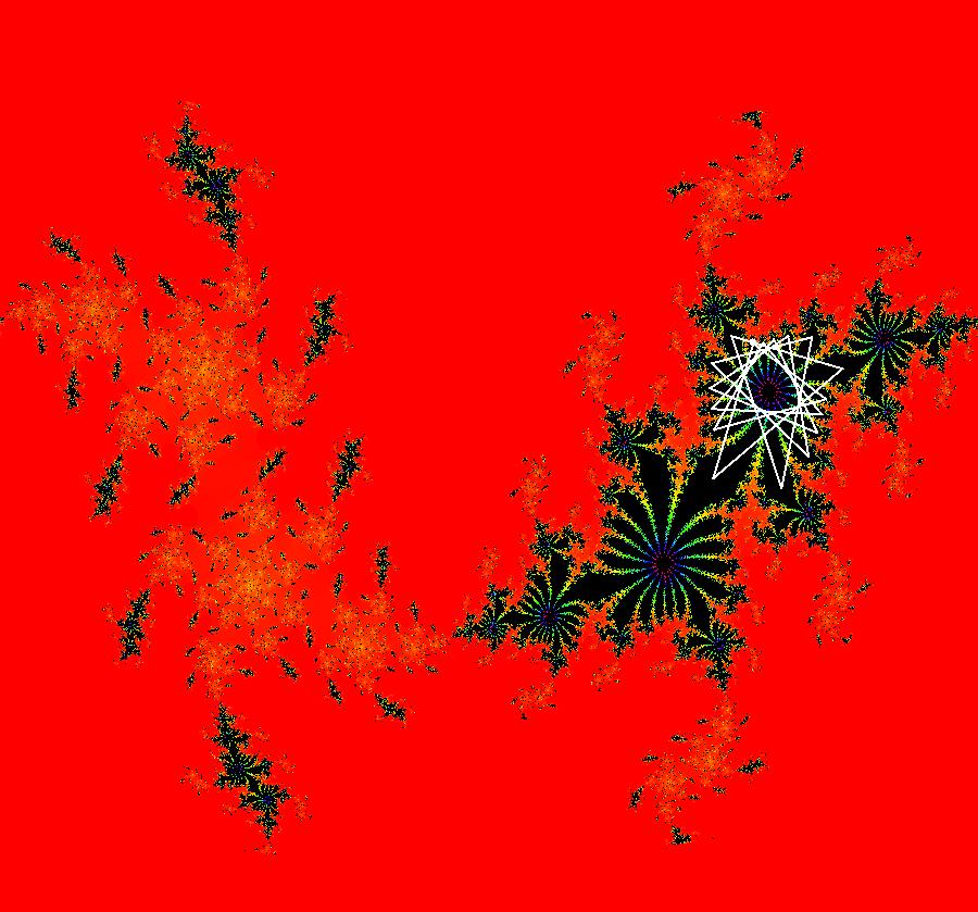
View/Sys/Gal: EMap "ComplexFns: EMap 1a, z <- z^2+c, c=.35+i*.35, per-34" in "VectorFields." This iteration is defined by: x <- p+x^2-y^2, y <- q+2*x*y. Parameters are: p = .3500; q = .3500; EMap CT: 0 Image 1: EMapMax view of the per-34 limit cycle.
|
|
|
View/Sys/Gal: EMap "ComplexFns: EMap 1a, z <- z^2+c, c=.36+i*0.11, no prisoner set" in "VectorFields." The complex system is: z <- z^2+c, with c = p+i*q, which generates the Mandelbrot fractals. The real system is defined by: x <- p+x^2-y^2, y <- q+2*x*y. Parameters are: p = .360; q = .110; There is no prisoner set. There are unstable fixed points at about: p1 = (.349064,.364392) and p2 = (.650936,-.364392). Image 1: EMapMax view after a Flow run with seed at p1. The orbit stays close to p1 for a while but after a hundred steps or so it spirals out to infinity. So - the black regions are not part of a prisoner set.
|
|
|
View/Sys/Gal: EMap "ComplexFns: EMap 1a, z <- z^2+c, c=.37+i*.33, per-5" in "VectorFields." This iteration is defined by: x <- p+x^2-y^2, y <- q+2*x*y. Parameters are: p = .3700; q = .3300; EMap CT: 0 This is a 5-petal fractal. Image 1: EMapMax view with the per-5 prisoner set limit cycle.
|
|
|
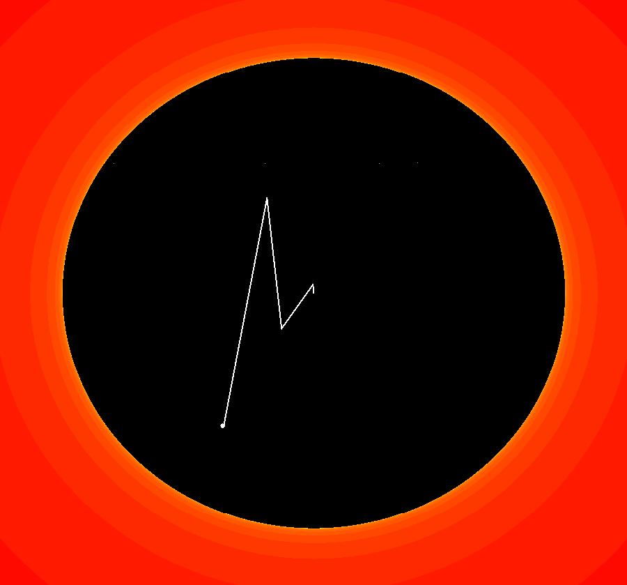
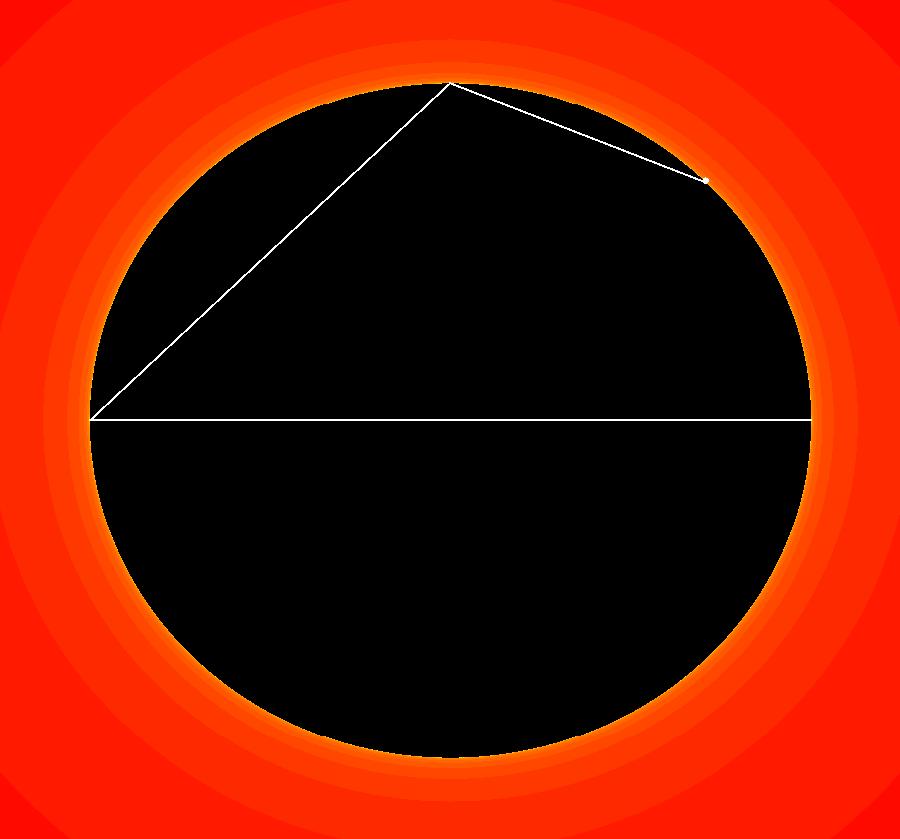
View/Sys/Gal: EMap "ComplexFns: EMap 1a, z <- z^2+c, c=0+i*0, per-1" in "VectorFields." This iteration is defined by: x <- p+x^2-y^2, y <- q+2*x*y. Parameters are: p = .0000; q = .0000; EMap CT: 0 The prisoner set is the unit disk. It has 2 fixed points: (0,0) and (1,0). Points inside the unit disk go to fixed point (0,0) and points on the edge of the disk go to fixed point (1,0). Image 1: EMap view with inside seed: (-.360429,-563209). Image 2: EMap view with edge seed: (.707107,.707107).
|
|
|
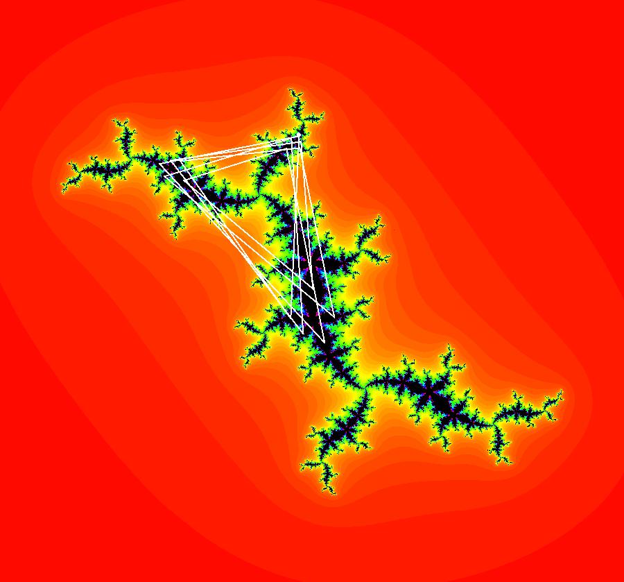
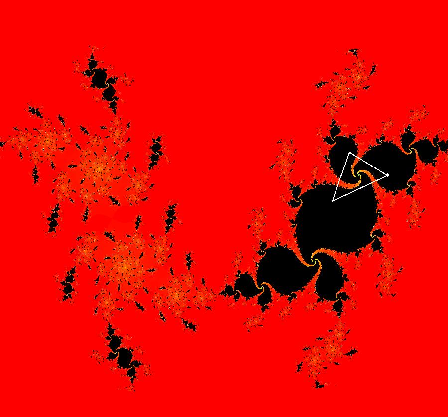
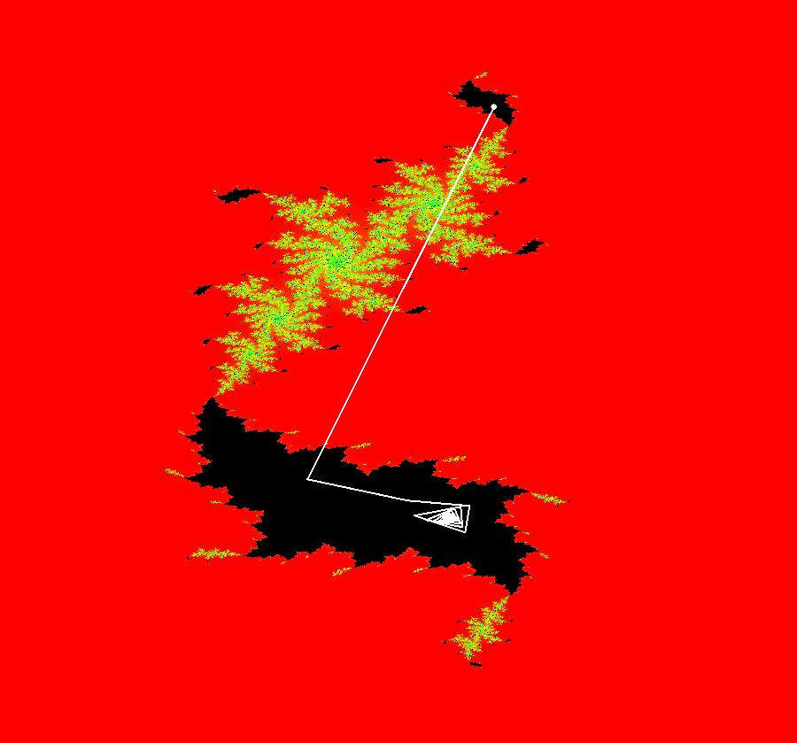
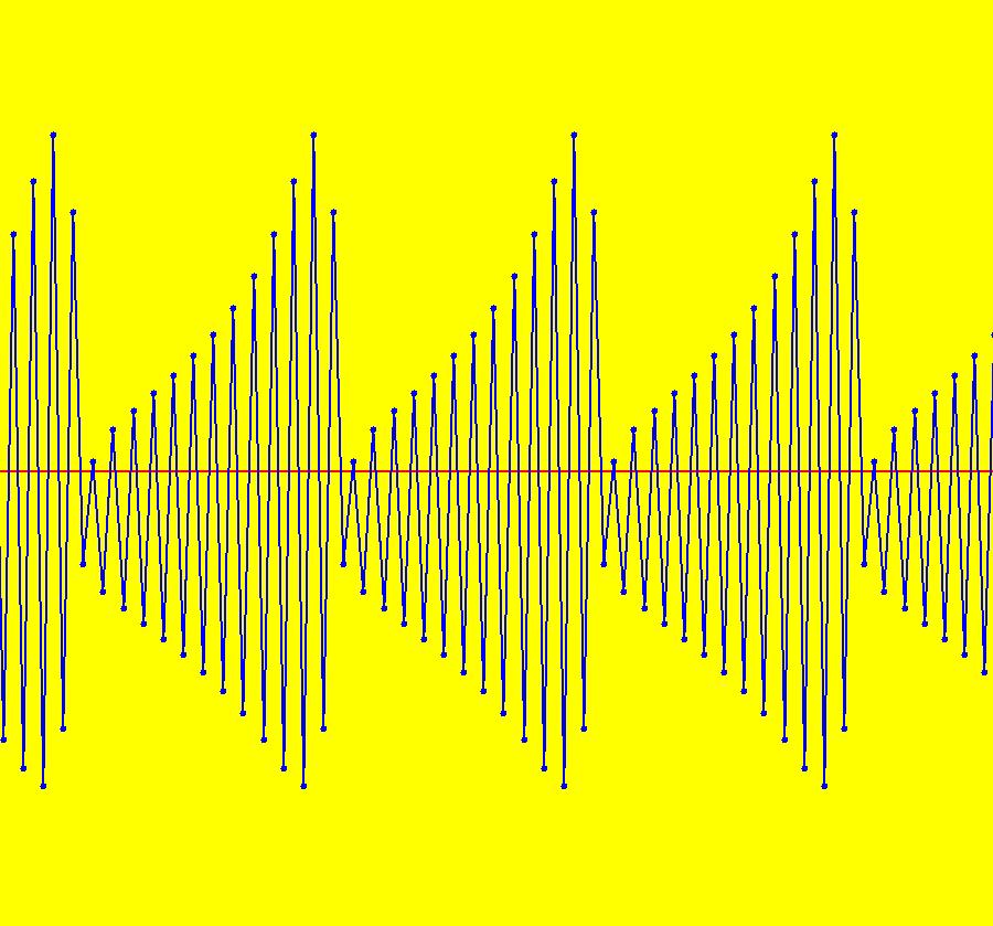
View/Sys/Gal: IMap "ComplexFns: EMap 1b, z <- z^2+c, c=.27+i*.57, per-4" in "VectorFields." This iteration is defined by: x <- x^2-y^2+p, y <- 2*x*y+q. Parameters are: p = .2700; q = .5700; EMap CT: 0 Go to the EMapMax view with "Show 2D IMap Orbit Sequence" on. Image 1: The per-4 limit cycle. Image 2: An orbit started in the prisoner set "outside" of the limit cycle. Image 3: An orbit started in the prisoner set "inside" of the limit cycle. NOTE: Limit cycles in Odes are continuous closed curves with an inside and an outside. Limit cycles in the IMap/EMap context are finite sequences of points so there is no inside and outside in the Ode sense. Image 4: The 3D/(t,x) IMap view.
|
|
|
View/Sys/Gal: EMap "ComplexFns: EMap 1b, z <- z^2+c, c=.310+i*.570, no prisoner set" in "VectorFields." This iteration is defined by: x <- x^2-y^2+p, y <- 2*x*y+q. Parameters are: p = .310; q = .570; Using the low resolution EMap setting seems to indicate that there may be some prisoner sets (the black regions). Image 1: EMap view. The higher resolution EMapMax setting shows that there really is no prisoner set for these values of p and q. Image 2: EMapMax view.
|
|
|
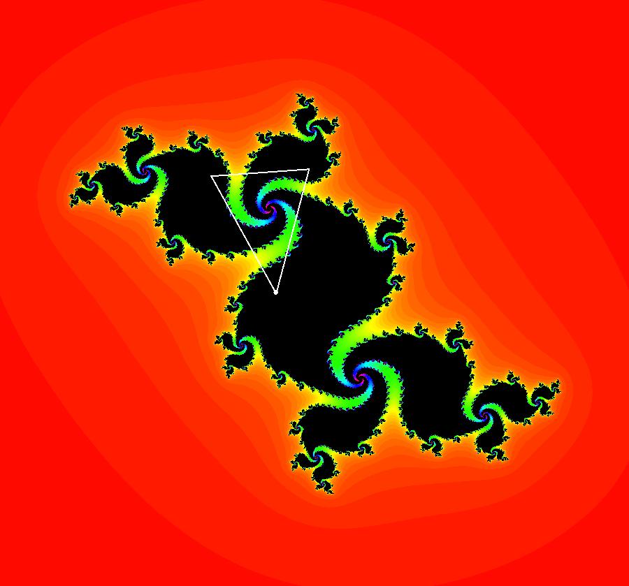
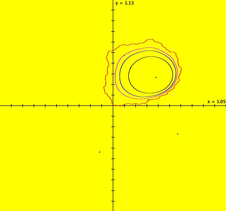
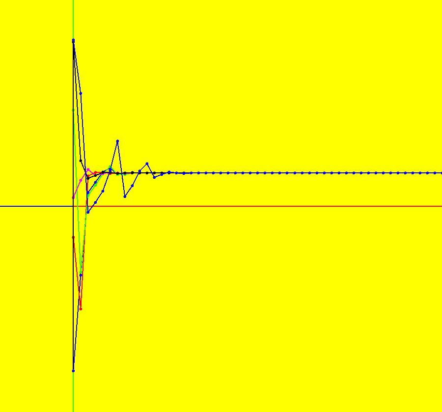
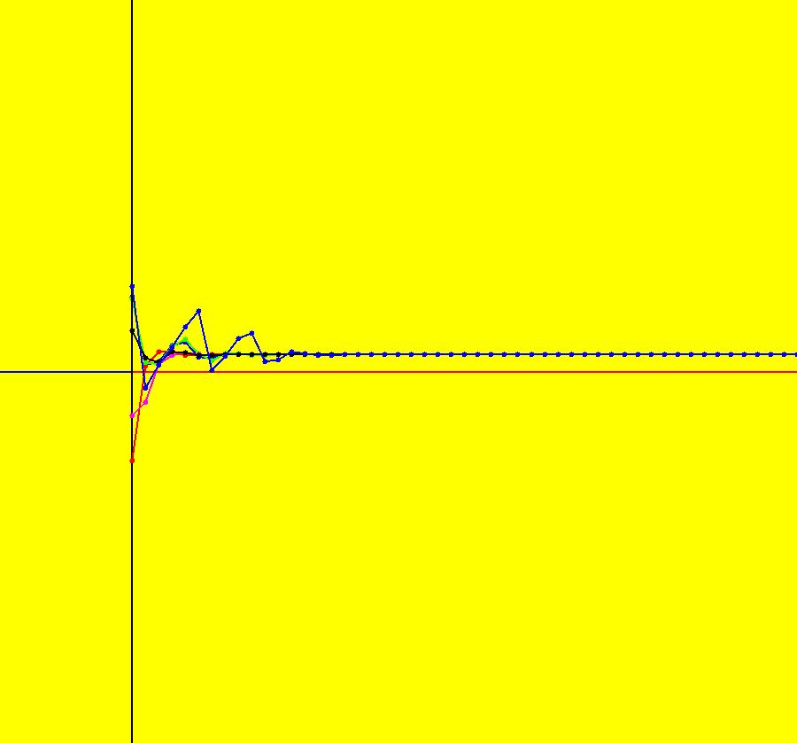
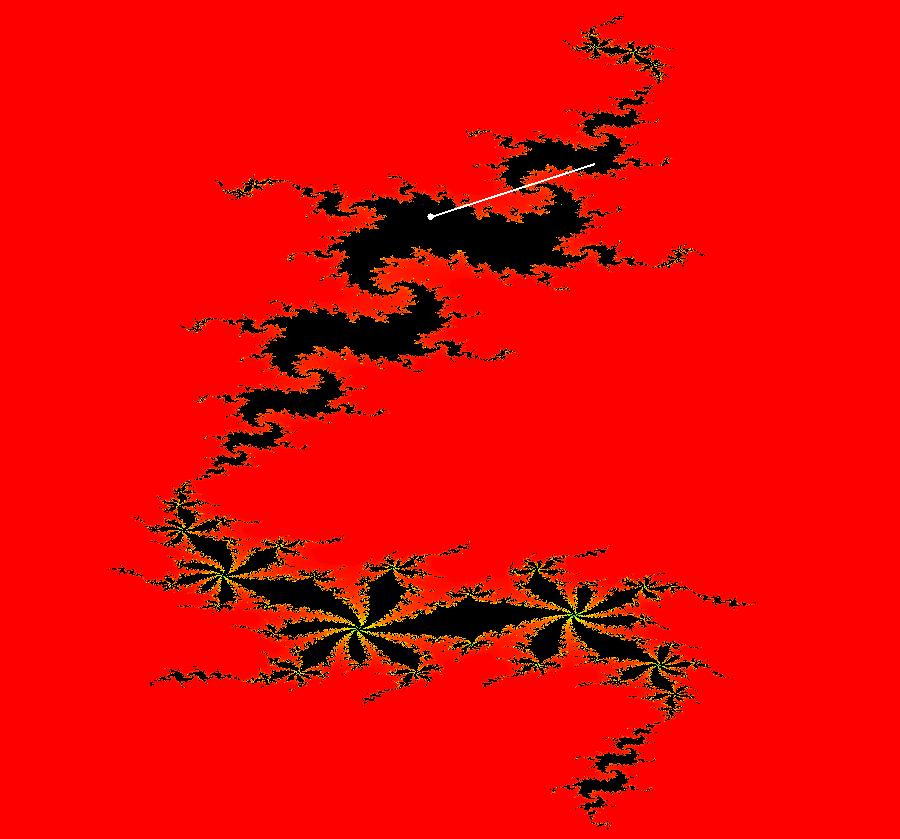
View/Sys/Gal: EMap "ComplexFns: EMap 1c, z <- z^2+c, c= .33+i*.06, chaotic attractors" in "VectorFields." This iteration is defined by: x <- p+x^2-y^2, y <- q+2*x*y. Parameters are: p = .33; q = .06; EMap CT: 0 There are fixed points in the prisoner set at (.4,.3) and (.6,-.3). Image 1: IMap view showing the two fixed points (black dots). The red curve is the outermost attractor. The magenta, black and blue curves are also attractors. The black curve is due to the seed at (-0.123558,-0.493744). Each prisoner set orbit, except for the two fixed points, goes to a different chaotic orbit in the large upper right lobe of the prisoner set. Image 2: EMap view after a Flow. See Sprott.
|
|
|
View/Sys/Gal: EMap "ComplexFns: EMap 2a, z <- r*z*(1-z), r=-.68-i*.74, per-19" in "VectorFields." This iteration is defined by: x <- p*x-p*x^2-q*y+2*q*x*y+p*y^2, y <- q*x-q*x^2+p*y-2*p*x*y+q*y^2. Parameters are: p = -.6800; q = -.7400; EMap CT: 0 Select "Show 2D IMap Orbit Sequence" to see the per-19 orbit. For a better image select "Show EMap w/Max Detail." Image 1: EMapMax view with per-19 limit cycle.
|
|
|
View/Sys/Gal: EMap "ComplexFns: EMap 2a, z <- r*z*(1-z), r=-.73-i*.73, per-8" in "VectorFields." This iteration is defined by: x <- p*x-p*x^2-q*y+2*q*x*y+p*y^2, y <- q*x-q*x^2+p*y-2*p*x*y+q*y^2. Parameters are: p = -.7200; q = -.7300; EMap CT: 0 Image 1: EMapMax view, per-8 limit cycle.
|
|
|
View/Sys/Gal: EMap "ComplexFns: EMap 2a, z <- r*z*(1-z), r=.87+i*.51, per-12" in "VectorFields." This iteration is defined by: x <- p*x-p*x^2-q*y+2*q*x*y+p*y^2, y <- q*x-q*x^2+p*y-2*p*x*y+q*y^2. Parameters are: p = .8700; q = .5100; EMap CT: 0 Image 1: EMapMax view, per-12 limit cycle.
|
|
|
View/Sys/Gal: EMap "ComplexFns: EMap 2a, z <- r*z*(1-z), r=.9+i*.48, no prisoner set" in "VectorFields." This iteration is defined by: x <- p*x-p*x^2-q*y+2*q*x*y+p*y^2, y <- q*x-q*x^2+p*y-2*p*x*y+q*y^2. Parameters are: p = .900; q = .480; This is a Mandelbrot fractal that has been scaled, rotated and shifted. The 2D Mandelbrot fractals and the 1D logistic map have the same symbolic form. Image 1: EMap view. The black regions are not really prisoner sets. Image 2: EMapMax view.
|
|
|
View/Sys/Gal: EMap "ComplexFns: EMap 2b, z <- r*z*(1-z), r=.89+i*.56, no prisoner set" in "VectorFields." This is another way to arrive at EMap 2a. The iteration is defined by: x <- p*F-q*G, y <- q*F+p*G. Parameters are: p = .890; q = .560; Functions are: F=x*(1-x)+y^2; G=y*(1-x)-x*y |
|
|
View/Sys/Gal: EMap "ComplexFns: EMap 2c, z <- r*z*(1-z), r=-.83+i*.55, per-1" in "VectorFields." This iteration is defined by: x <- p*F-q*G, y <- q*F+p*G. Parameters are: p = -.8300; q = .5500; Functions are: F=x*(1-x)+y^2; G=y*(1-x)-x*y EMap CT: 0 Image 1: EMapMax view. Every prisoner set orbit goes to the fixed point at (0,0).
|
|
|
View/Sys/Gal: EMap "ComplexFns: EMap 2c, z <- r*z*(1-z), r=.21+i*.99, no prisoner set" in "VectorFields." This iteration is defined by: x <- p*x-p*x^2-q*y+2*q*x*y+p*y^2, y <- q*x-q*x^2+p*y-2*p*x*y+q*y^2. Parameters are: p = .210; q = .990; Image 1: EMap view. Image 2: The EMapMax view shows that there is no set.
|
|
|
View/Sys/Gal: EMap "ComplexFns: EMap 2c, z <- r*z*(1-z), r=.21+i*.99, no prisoner set" in "VectorFields." This iteration is defined by: x <- p*x-p*x^2-q*y+2*q*x*y+p*y^2, y <- q*x-q*x^2+p*y-2*p*x*y+q*y^2. Parameters are: p = .210; q = .990; Image 1: EMap view. Image 2: The EMapMax view shows that there is no prisoner set.
|
|
|
View/Sys/Gal: EMap "ComplexFns: EMap 2c, z <- r*z*(1-z), r=.31+.99, per-5" in "VectorFields." This iteration is defined by: x <- p*x-p*x^2-q*y+2*q*x*y+p*y^2, y <- q*x-q*x^2+p*y-2*p*x*y+q*y^2. Parameters are: p = .3100; q = .9900; EMap CT: 0 Image 1: EMapMax view. The per-5 limit cycle attractor for all prisoner set orbits.
|
|
|
View/Sys/Gal: EMap "ComplexFns: EMap 2d, z <- r*z*(1-z), r=.900+i*.500, no prisoner set" in "VectorFields." This iteration is defined by: x <- p*x-p*x^2-q*y+2*q*x*y+p*y^2, y <- q*x-q*x^2+p*y-2*p*x*y+q*y^2. Parameters are: p = .900; q = .500; Image 1: EMap view. No prisoner set.
|
|
|
View/Sys/Gal: EMap "ComplexFns: EMap 2e, z <- z*(1-z)+c, c=.91-i*.38, no prisoner set" in "VectorFields." This iteration is defined by: x <- p+x-x^2+y^2, y <- q+y-2*x*y. Parameters are: p = .910; q = -.380; Image 1: EMap view. Again no prisoner set.
|
|
|
View/Sys/Gal: EMap "ComplexFns: EMap 3a, z <- sin(z)+c, c=-4.200+i*1.000, no prisoner set" in "VectorFields." This iteration is defined by: x <- sin(x)*cosh(y)+p, y <- cos(x)*sinh(y)+q. Parameters are: p = -4.200; q = 1.000; This EMap extends to +/- infinity in the x direction. Image 1: EMap view. No prisoner set.
|
|
|
View/Sys/Gal: EMap "ComplexFns: EMap 3a, z <- sin(z)+c, c=-4.3+i*1, per-11" in "VectorFields." This iteration is defined by: x <- sin(x)*cosh(y)+p, y <- cos(x)*sinh(y)+q. Parameters are: p = -4.3000; q = 1.0000; EMap CT: 0 Image 1: EMapMax view with per-11 prisoner set.
|
|
|
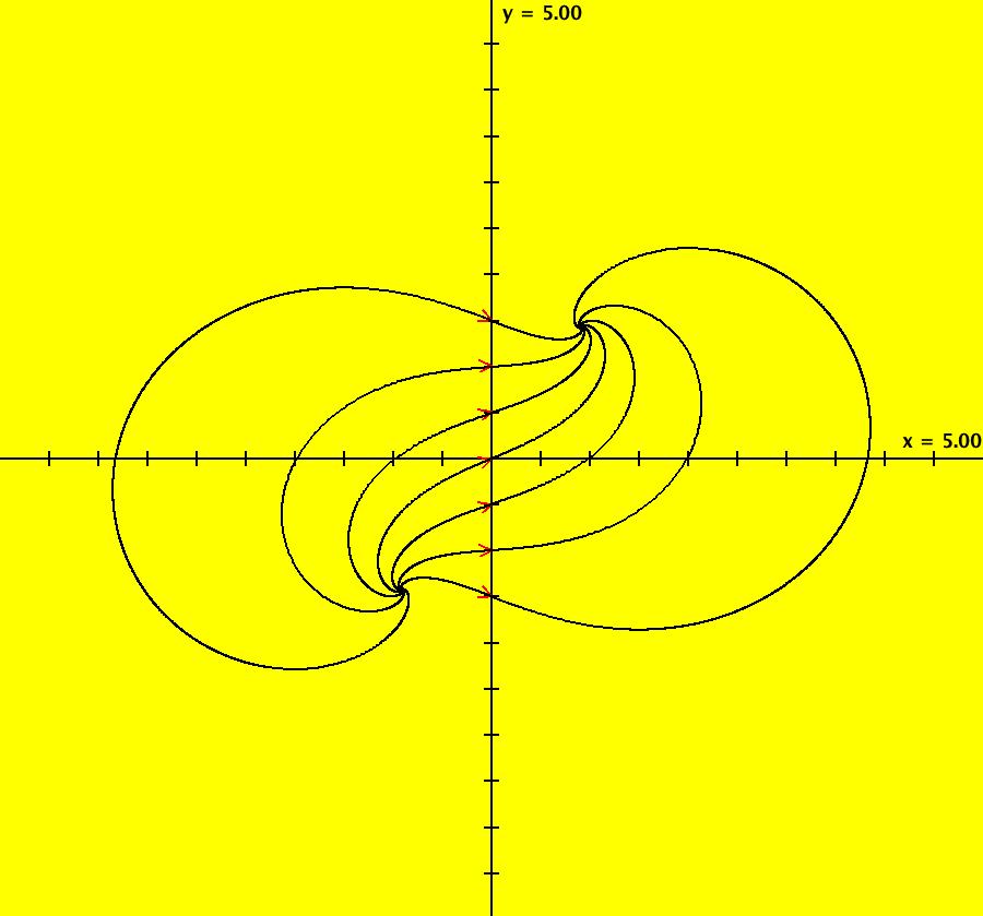
View/Sys/Gal: IMap "ComplexFns: EMap 3b, z <- sin(z)+c, c=.5+i*.5, per-1" in "VectorFields." This iteration is defined by: x <- sin(x)*cosh(y)+p, y <- cos(x)*sinh(y)+q. Parameters are: p=.5; q=.5 This EMap extends to +/- infinity in the x direction. Turn "Show 2D IMap Orbit Sequence" on. All orbits starting in the prisoner set seem to converge to the fixed point: (x,y) = (1.615291,0.477923). Image 1: EMap view. Extend hMax to 50 and go to the 3D IMap view. Image 2: 3D/(t,x) IMap view, with 6 orbits starting in the prisoner set. Image 3: 3D/(t,y) IMap view, with 6 orbits starting in the prisoner set.
|
|
|
View/Sys/Gal: EMap "ComplexFns: EMap 3c, z <- (1+s*.1)*(sin(z)+c), c=-.18+i*.5, s=5.9, per-11" in "VectorFields." This iteration is defined by: x <- (1+s*.1)*(sin(x)*cosh(y)+p), y <- (1+s*.1)*(cos(x)*sinh(y)+q). Parameters are: p = -.1800; q = .5000; s = 5.9000; EMap CT: 0 Select "Show 2D IMap Orbit Sequence" to see the orbit. For these values of p, q and s, all orbits starting in the black prisoner set are asymptotic to the period 11 orbit starting at (-1.591794,-0.000000). The EMap image itself is periodic in the x direction. To see this, zoom out. Image 1: EMapMax with per-11 prisoner set limit cycle.
|
|
|
View/Sys/Gal: EMap "ComplexFns: EMap 3c, z <- (1+s*.1)*(sin(z)+c), c=.08+i*.52, s=5.9, per-3" in "VectorFields." This is basically a time-scaled version of: z <- sin(z)+c. This iteration is defined by: x <- (1+s*.1)*(sin(x)*cosh(y)+p), y <- (1+s*.1)*(cos(x)*sinh(y)+q). Parameters are: p = .0800; q = .5200; s = 5.9000; EMap CT: 0 To see the periodic orbit select "Show 2D IMap Orbit Sequence" on the Settings menu. For these parameter values, all orbits starting in the black prisoner set are asymptotic to the period 3 orbit through the points: (x1,y1) = (2.285781094122398,0.5498791196477172), (x2,y2) = (1.513947184769878,0.22427256545863153), (x3,y3) = (1.7547214652461967,0.8472313873170241). Image 1: EMapMax view with per-3 limit cycle. The EMap image itself is periodic with period 2 π in the x direction. To see this, zoom out.
|
|
|
View/Sys/Gal: EMap "ComplexFns: EMap 3c, z <- (1+s*.1)*(sin(z)+c), c=.12+i*.49, s=6.1, per-17" in "VectorFields." This iteration is defined by: x <- (1+s*.1)*(sin(x)*cosh(y)+p), y <- (1+s*.1)*(cos(x)*sinh(y)+q). Parameters are: p = .1200; q = .4900; s = 6.1000; EMap CT: 0 Select "Show 2D IMap Orbit Sequence" to see the orbit. For these values of p, q and s, all orbits starting in the black prisoner set are asymptotic to the period 17 orbit starting at (1.802709,0.788560). Image 1: EMapMax view with per-17 prisoner set limit cycle. The EMap image itself is periodic in the x direction. To see this, zoom out.
|
|
|
View/Sys/Gal: EMap "ComplexFns: EMap 4a, z <- e^z+c, c=.3+i*.83, per-7" in "VectorFields." This iteration is defined by: x <- e^x*cos(y)+p, y <- e^x*sin(y)+q. Parameters are: p = .3000; q = .8300; EMap CT: 0 The prisoner set is infinite, disconnected and periodic in the y direction with period 2 π. All orbits starting in the prisoner set go to a single per-7 orbit. Image 1: EMapMax, prisoner set with per-7 limit cycle. Image 2: An Art image. EmapMaxCT5 zoomed in 6X at (.0343673,1.8303076).
|
|
|
View/Sys/Gal: EMap "ComplexFns: EMap 4a, z <- e^z+c, c=.310+i*.830, no prisoner set" in "VectorFields." This iteration is defined by: x <- e^x*cos(y)+p, y <- e^x*sin(y)+q. Parameters are: p = .310; q = .830; From z <- e^z+(p+i*q). This EMap also extends to +/- infinity in the y direction. Image 1: EMap view. Another interesting Art image but there is no prisoner set for these parameter values. Image 2: EMapMax view. No prisoner set Image 3: Center at (.1116,1.84828) and zoom in 4X. Get into the EMapMaxCT5 view.
|
|
|
View/Sys/Gal: EMap "ComplexFns: EMap 5, z <- e^z+z*(1-z)+c, c=-1.1+i*.19, per-1" in "VectorFields." This iteration is defined by: x <- p+x-x^2+y^2+e^x*cos(y), y <- q+y-2*x*y+e^x*sin(y). Parameters are: p = -1.100; q = .190; Is this the entire image? All orbits starting in the prisoner set seem to go to the fixed point (x,y) = (1.251157,-1.248730). Image 1: EMapMax view showing a prisoner set orbit going to the fixed point.
|
|
|
View/Sys/Gal: IMap "ComplexFns: EMap 5b, z <- e^z+z*(1-z)+c, c=-1.1+i*.31, per-7 and 2" in "VectorFields." This iteration is defined by: x <- p+x-x^2+y^2+e^x*cos(y), y <- q+y-2*x*y+e^x*sin(y). Parameters are: p = -1.1000; q = .3100; EMap CT: 0 There are 2 basic fractals here: 2-petal and 7-petal spiral fractals. The tails of the 2-petal spirals are 7-petal spirals and vice versa. The 2-petal spirals are asymptotic to a per-2 orbit and the 7-petal spirals are asymptotic to a per-7 orbit. Image 1: EMapMax view with a per-2 limit cycle. Image 2: IMap view showing the per-2 (red) and per-7 (blue) limit cycles.
|
|
|
View/Sys/Gal: EMap "ComplexFns: EMap 5c, z <- e^z+z*(1-z)+c, c=-1+i*.048, per-10" in "VectorFields." This iteration is defined by: x <- p+x-x^2+y^2+e^x*cos(y), y <- q+y-2*x*y+e^x*sin(y). Parameters are: p = -1.0000; q = .0480; EMap CT: 0 All prisoner set orbits go to a per-10 limit cycle. Image 1: EMapMax view.
|
|
|
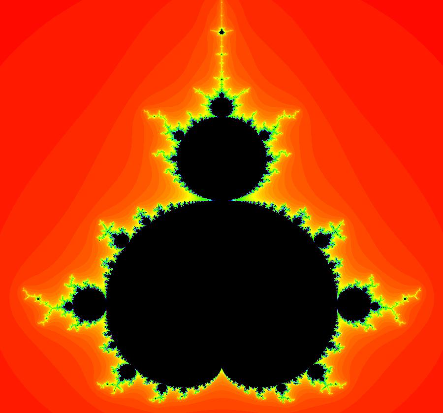
View/Sys/Gal: EMap "ComplexFns: EMap 6, z <- e^z+sin(z)+c, bifurcation diagram" in "VectorFields." This system of odes is defined by the equations: dx/dt = x, dy/dt = y, dz/dt = x+e^z*cos(w)+cosh(w)*sin(z), dw/dt = y+e^z*sin(w)+cos(z)*sinh(w). This is the bifurcation diagram of system 6: z <- e^z+sin(z)+c, where c = p+i*q. Read "x" as "p" and "y as "q." The image is in the parameter space, not the phase space, of system 6: z <- e^z+sin(z)+c. If the system were z <- z^2+c the image would be the Mandelbrot set. Image 1: EMap view of the bifurcation diagram for: z <- e^z+sin(z)+c.
|
|
|
View/Sys/Gal: EMap "ComplexFns: EMap 6, z <- e^z+sin(z)+c, c=-.36+i*.16, per-8, disconnected prisoner set" in "VectorFields." This iteration is defined by: x <- p+e^x*cos(y)+cosh(y)*sin(x), y <- q+e^x*sin(y)+cos(x)*sinh(y). Parameters are: p = -.3600; q = .1600; EMap CT: 0 The EMapMax view shows that the prisoner set is disconnected for this example. All prisoner set orbits go to a per-8 limit cycle. Image 1: EMapMax view. The orbit on the small prisoner set island at (0.135675,0.362270) goes to the per-8 limit cycle. Image 2: A zoomed in view of the small island.
|
|
|
View/Sys/Gal: EMap "ComplexFns: EMap 6, z <- e^z+sin(z)+c, c=-.38+i*.11, no prisoner set" in "VectorFields." This iteration is defined by: x <- p+e^x*cos(y)+cosh(y)*sin(x), y <- q+e^x*sin(y)+cos(x)*sinh(y). Parameters are: p = -.380; q = .110; This EMap image is repeated on the interval from -infinity to about 2 in the x direction. Switching to EMapMax shows that there is no prisoner set for this system. Image 1: EMap view. Zoom in on a small blip. Image 2: EMap of a blip, zoomed in.
|
|
|
View/Sys/Gal: EMap "ComplexFns: EMap 6, z <- e^z+sin(z)+c, c=-.38+i*.12, per-9" in "VectorFields." This iteration is defined by: x <- p+e^x*cos(y)+cosh(y)*sin(x), y <- q+e^x*sin(y)+cos(x)*sinh(y). Parameters are: p = -.3800; q = .1200; EMap CT: 0 Image 1: EMapMax view with per-9 prisoner set limit cycle. Again we have a disconnected prisoner set. The prisoner set is also periodic in the -x direction. Here we have a fractal with disconnected parts. The small black islands are copies of the main image or parts of the main image. Image 2: Zoomed in on an island.
|
|
|
View/Sys/Gal: EMap "ComplexFns: EMap 6, z <- e^z+sin(z)+c, c=-.4+i*.75, per-4" in "VectorFields." This iteration is defined by: x <- p+e^x*cos(y)+cosh(y)*sin(x), y <- q+e^x*sin(y)+cos(x)*sinh(y). Parameters are: p = -.4000; q = .7500; EMap CT: 0 Image 1: EMapMax image with prisoner set per-4 limit cycle. Image 2: A fractal island.
|
|
|
View/Sys/Gal: EMap "ComplexFns: EMap 6, z <- e^z+sin(z)+c, c=-.4+i*0.9, per-10" in "VectorFields." This iteration is defined by: x <- p+e^x*cos(y)+cosh(y)*sin(x), y <- q+e^x*sin(y)+cos(x)*sinh(y). Parameters are: p = -.4000; q = .0900; EMap CT: 0 Image 1: The EMapMax per-10 limit cycle attractor for prisoner set orbits. This system has an infinite number of unstable fixed points. They are located where the 10-petal parts of the image come together. For example, there is an unstable fixed point inside the limit cycle at about: (x,y) = (-1.0864,.4391).
|
|
|
View/Sys/Gal: EMap "ComplexFns: EMap 6, z <- e^z+sin(z)+c, c=-2.5+i*.9, per-34" in "VectorFields." This iteration is defined by: x <- p+e^x*cos(y)+cosh(y)*sin(x), y <- q+e^x*sin(y)+cos(x)*sinh(y). Parameters are: p = -2.5000; q = .9000; EMap CT: 0 Image 1: EMapMax image with prisoner set per-34 limit set. There are 17-petal and 2-petal fractals. The 34 comes from 2*17. Image 2: Zoomed in on a fractal island.
|
|
|
View/Sys/Gal: EMap "ComplexFns: EMap 7, z <- sin(z)+cos(z)+c, c=.6+i*.17, per-2" in "VectorFields." This iteration is defined by: x <- p+cos(x)*cosh(y)+cosh(y)*sin(x), y <- q+cos(x)*sinh(y)-sin(x)*sinh(y). Parameters are: p = .6000; q = .1700; EMap CT: 0 Image 1: EMap view showing the prisoner set per-2 limit cycle.
|
|
|
View/Sys/Gal: IMap "ComplexFns: EMap 7, z <- sin(z)+cos(z)+c, c=.6+i*.26, per-48" in "VectorFields." This iteration is defined by: x <- p+cos(x)*cosh(y)+cosh(y)*sin(x), y <- q+cos(x)*sinh(y)-sin(x)*sinh(y). Parameters are: p = .6000; q = .2600; EMap CT: 0 Image 1: EMapMax on with the per-48 limit cycle prisoner set orbit. There are 2 petal and 12 petal floral fractal components in the image. We see that each of the 12 petals are visited twice so the 48 comes from 2*(2*12). Image 2: 3D/(t,y) IMap view of the per-48 orbit with hMin = .54, hMax = 100.
|
|
|
View/Sys/Gal: EMap "ComplexFns: EMap 7, z <- sin(z)+cos(z)+c, c=.6-i*.24, per-26" in "VectorFields." This iteration is defined by: x <- p+cos(x)*cosh(y)+cosh(y)*sin(x), y <- q+cos(x)*sinh(y)-sin(x)*sinh(y). Parameters are: p = .6000; q = -.2400; EMap CT: 0 Here we have 2-petal and 13-petal spiral fractals which cause the 2*13 = 26 period prisoner set limit cycle. Image 1: EMapMax view with the per-26 prisoner set limit cycle. Image 2: 3D/(t,y) IMap view of the per-26 prisoner set limit cycle (hMax = 100).
|
|
|
View/Sys/Gal: IMap "ComplexFns: EMap 7, z <- sin(z)+cos(z)+c, c=.6-i*.24, per-26" in "VectorFields." This iteration is defined by: x <- p+cos(x)*cosh(y)+cosh(y)*sin(x), y <- q+cos(x)*sinh(y)-sin(x)*sinh(y). Parameters are: p = .6000; q = -.2400; EMap CT: 0 Here we have 2-petal and 13-petal spiral fractals which cause the 2*13 = 26 period prisoner set limit cycle. Image 1: EMapMax view with the per-26 prisoner set limit cycle. Image 2: 3D/(t,y) IMap view of the per-26 prisoner set limit cycle (hMax = 100).
|
|
|
View/Sys/Gal: EMap "ComplexFns: EMap 7, z <- sin(z)+cos(z)+c, c=1+i*.64, per-2" in "VectorFields." This iteration is defined by: x <- p+cos(x)*cosh(y)+cosh(y)*sin(x), y <- q+cos(x)*sinh(y)-sin(x)*sinh(y). Parameters are: p = 1.0000; q = .6400; EMap CT: 0 This system consists of 2-petal fractals. The prisoner set is not connected. There is a per-2 prisoner set limit cycle. Image 1: EMapMax view with a seed in a disconnected part of the prisoner set. The orbit goes to the per-2 limit cycle. Image 2: The per-2 limit cycle.
|
|
An OdeFactory Slide Show Click on a slide to zoom in. Click "video" to see a video. |
View/Sys/Gal: Ode "NonAutonToAutonExs: ***** Introduction *****" in "VectorFields." ***** Introduction ***** This algorithm for the conversion of a nonautonomous system of odes, or iterations, to an autonomous system consists of promoting each state variable to the next state variable and adding dx/dt = 1 to the system. Algorithm: prepend dx/dt = 1 to the system then promote (t,x,y) to (x,y,z) in the old system dx/dt = 1, dx/dt = f(t,x,y) -> dy/dt = f(x,y,z), dy/dt = g(t,x,y) -> dz/dt = g(x,y,z). Note: using dx/dt = 1 gives a new IMap for the 3D system and using x <- x+1 gives a new Ode for the 3D system.
|
|
|
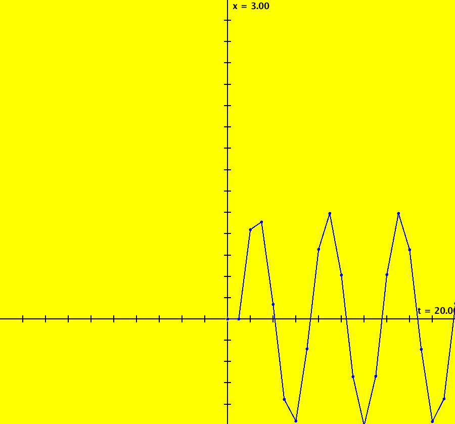
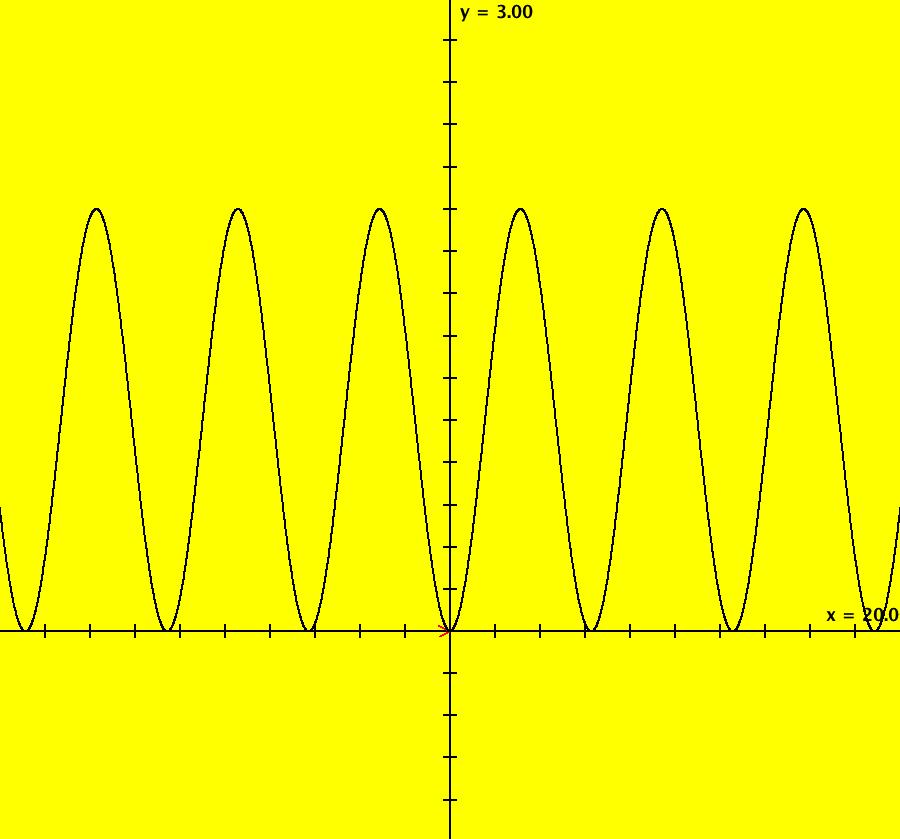
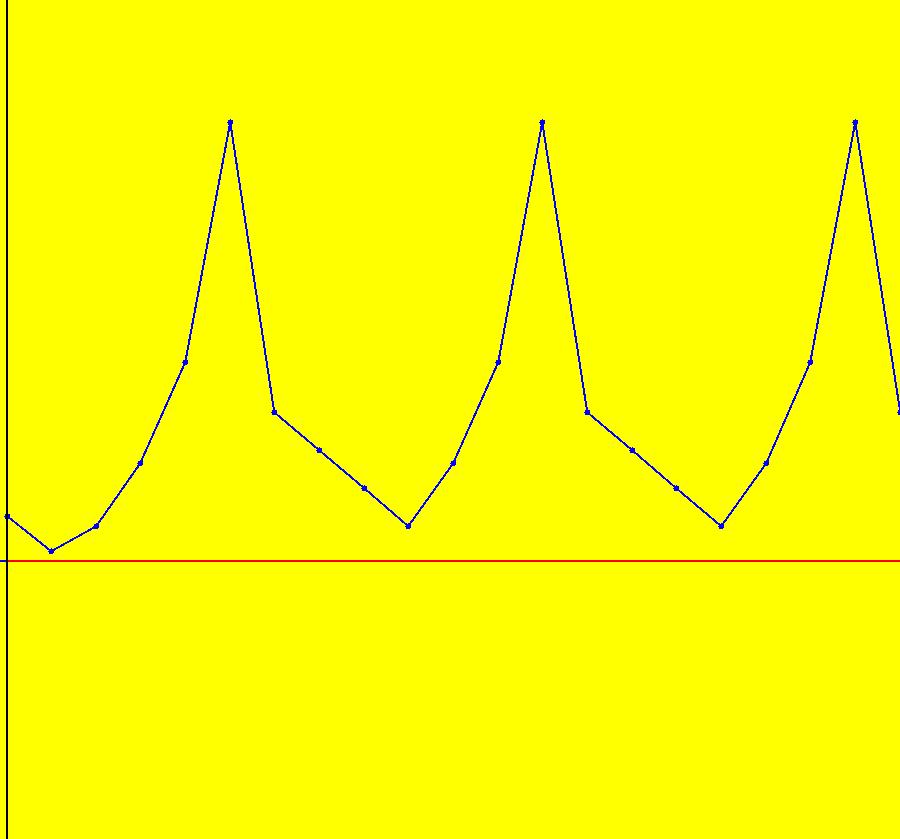
View/Sys/Gal: IMap "NonAutonToAutonExs: (A) 1D NonAuton (d*sin(t)), d=1" in "VectorFields." This ode is defined by the equation: dx/dt = d*sin(t) in the (t,x) coordinate system. Parameters are: d=1 ICs: (t,x) = (0,0). Image 1: Ode view. Image 2: IMap view. The 2D nonautonomous Ode system would be: dx/dt = 1, dy/dt = d*sin(x) or, for the same IMap view, x <- x+1, y <- d*sin(x).
|
|
|
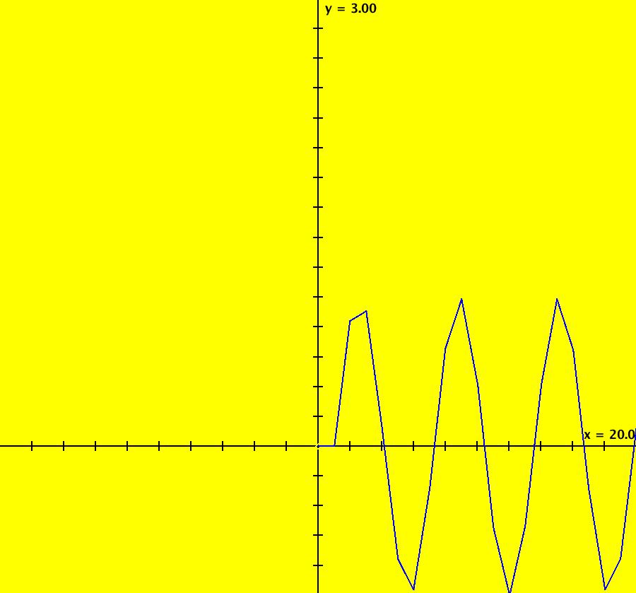
View/Sys/Gal: IMap "NonAutonToAutonExs: (B) 2D Auton Ode-equivalent ver (1,d*sin(x)), d=1" in "VectorFields." This system of odes is defined by the equations: dx/dt = 1, dy/dt = d*sin(x). Parameters are: d=1 ICs: (t,x,y) = (0,0,0). Image 1: Ode view. Image 2: IMap1000 view. Same as the 1D version in the Ode view - but different in the IMap1000 view.
|
|
|
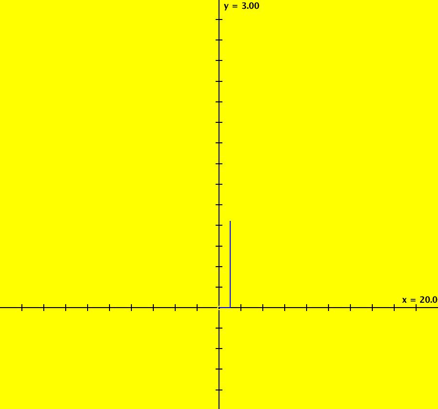
View/Sys/Gal: Ode "NonAutonToAutonExs: (C) 2D Auton IMap1000-equivalent ver (x+1,d*sin(x)), d=1" in "VectorFields." This iteration is defined by: x <- x+1, y <- d*sin(x). Parameters are: d=1 ICs: (t,x,y) = (0,0,0). Image 1: IMap view. Image 2: Ode view. Same as the 1D version in the IMap view - but different in the Ode view.
|
|
|
View/Sys/Gal: IMap "NonAutonToAutonExs: (D) 2D NonAuton (y,-k*sin(x)-c*y+d*sin(t)), k = 1.100; c = .040; d = .370;" in "VectorFields." This system of odes is defined by the equations: dx/dt = y, dy/dt = -k*sin(x)-c*y+d*sin(t) in the (t,x,y) coordinate system. Parameters are: k = 1.100; c = .040; d = .370; In the (x,y) view, the ICs are: (t,x,y) = (0,1,0). Image 1: Ode view. Image 2: IMap view. The corresponding 3D autonomous system is: dx/dt = 1,
dy/dt = z, dz/dt = -k*sin(y)-c*z+d*sin(x).
|
|
|
View/Sys/Gal: Ode "NonAutonToAutonExs: (E) 3D Auton Ode-equivalent ver (1,z,-k*sin(y)-c*z+d*sin(x)), k = 1.100; c = .040; d = .370;" in "VectorFields." This system of odes is defined by the equations: dx/dt = 1, dy/dt = z, dz/dt = -k*sin(y)-c*z+d*sin(x). Parameters are: k = 1.100; c = .040; d = .370; In the (y,z) view, the ICs are: (t,x,y,z) = (0,0,1,0). Image 1: Ode view.
|
|
|
View/Sys/Gal: Ode "NonAutonToAutonExs: (F) 3D Auton IMap-equivalent ver (x+1,z,-k*sin(y)-c*z+d*sin(x)), k = 1.100; c = .040; d = .370;" in "VectorFields." This system of odes is defined by the equations: x <- x+1, y <- z, z <- -k*sin(y)-c*z+d*sin(x). Parameters are: k = 1.100; c = .040; d = .370; In the (y,z) view, the ICs are: (t,x,y,z) = (0,0,1,0). Image 1: IMap view. Same as the 2D version in the IMap view - but new and different in the Ode view. Image 2: Ode view.
|
|
|
View/Sys/Gal: IMap "NonAutonToAutonExs: (G) 3D Auton new IMap1001, Art image" in "VectorFields." This system of odes is defined by the equations: dx/dt = 1, dy/dt = z, dz/dt = -k*sin(y)-c*z+d*sin(x). Parameters are: k = 1.100; c = .049; d = .390; This Art image uses the new IMap generated from the Ode-equivalent version of the 2D nonautonomous system. Parameter c has been changed from .040 to .049 and parameter d has been changed from .370 to .390. Image 1: IMap view.
|
|
An OdeFactory Slide Show Click on a slide to zoom in. Click "video" to see a video. |
View/Sys/Gal: Ode "PMFn: ***** Introduction *****" in "VectorFields." ***** Introduction ***** The purpose of this section is to study the iteration of a function defined in the OdeFactory program by a bit manipulation algorithm. The function, which I call pm(x), is a Java variation of a Post Machine (PM for short) example given in Feynman's book, "Lectures on Computation," p. 92. PMs are of interest because they are equivalent to Universal Turing Machines.
Feynman's example function, which I will call PMA(str), involves the manipulation of a finite bit string by a PM program. The string is the data. The algorithm PMA(str) is the PM's program which Feynman does not give explicitly. Feynman defines PMA(str) as follows. For a finite string of bits called str, if str starts with a 1 append 1101 else append 00. Delete the first three bits of str and return the new str. For example: str = 10010 -> 101101 -> 1011101 ... I wrote a Java variation of the algorithm, called pm(x), which can be used in OdeFactory to study the iteration. Inputs to OdeFactory are Java doubles, not strings, so a double x needs to be converted to a binary string str, then PMA(str) needs to be applied to the string and the result needs to be returned as a double. Suppose x is a Java double which defines the input string. To get the next iterate of x, pm(x), we need to apply the following steps: (1) scale x and convert it to a long int xLong = (long)(x*100+0.0000001); (2) convert the xLong to a binary string str = Long.toString(xLong,2); (3) apply PMA to str to get newStr (4) convert newStr to a long int xLong = Long.parseLong(strNew,2); (5) unscale xLong and return a double return (double)xLong/100; There are some differences between PMA(str) and pm(y). Without the 0.0000001, step (1) can give an incorrect result. For example, 4.77 becomes 469 since internally: 4.77*100 is 469.999...94, not 477. In step (4) any leading 0's of strNew will be lost. For example: Long.parseLong("01001",2) and Long.parseLong("1001",2) both give 9. Consequently, str always starts with a 1. pm(x) is defined, in words, as follows: For the finite string of bits, str, representing x*100 as a Java long int, append 1101 then delete the first three bits of str and return strNew as a Java double. So pm(x) is not the same as PMA(str). It is a Java variation of PMA(str).
|
|
|
View/Sys/Gal: IMap "PMFn: (2) (r*pm(x)), r=1 IMap1100" in "VectorFields." This iteration is defined by: x <- r*pm(x). Parameters are: r=1 The seed is at (0,.18). Image 1: IMap view, x = .18 -> a fixed point at x = 4.77. Vary r to find a 7-cycle.
|
|
|
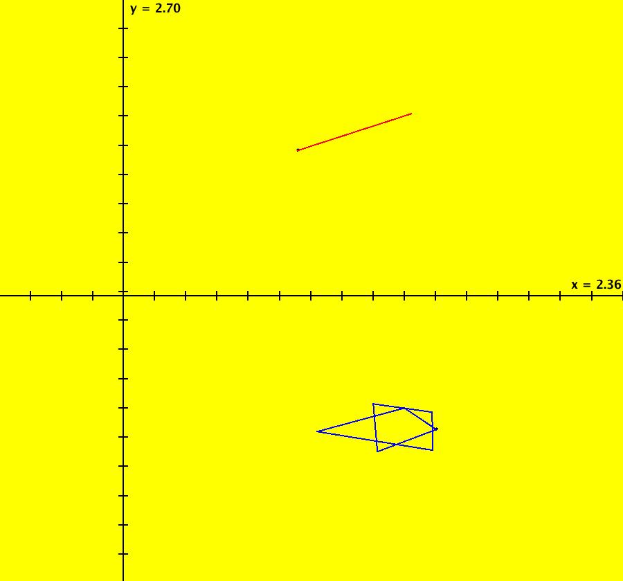
View/Sys/Gal: IMap "PMFn: (3) (x,x*pm(y)) IMap1100" in "VectorFields." This iteration is defined by: x <- x, y <- x*pm(y). Variable x plays the role of parameter r in system (2) and variable y plays the role of x in system (2). The seed, shown by the black dot at (x,y) = (1.4,.18), gives a 7-cycle. Start a Flow. Image 1: IMap orbit in the 2D/(x,y) view. Since x <- x the motion is in the y direction only. Image 2: The IMap 3D/(t,y) view shows the 7-cycle.
|
|
|
View/Sys/Gal: EMap "PMFn: (4) ((1+s*.1)*x,(1+s*.1)*x*pm(y)), s = .021; EMapCT3" in "VectorFields." This iteration is defined by: x <- (1+s*.1)*x, y <- (1+s*.1)*x*pm(y). Parameters are: s = .021; It is a time-scaled version of system (3). Image 1: EMap view w/CT 7, s = .021. The EMap is the Feigenbaum bifurcation diagram of system (2). Vary s. Try different color tables.
|
|
An OdeFactory Slide Show Click on a slide to zoom in. Click "video" to see a video. |
View/Sys/Gal: Ode "QuasiHamiltonian: ***** Introduction *****" in "VectorFields." ***** Introduction ***** Suppose we want to create a system of odes that has trajectories on the curve: H(x,y) = 0. Setting: dx/dt = Hy, dy/dt = -Hx gives the desired system. The system is called a Hamiltonian system and H(x,y) is called the Hamiltonian function (H is the total energy in a Physics context). If H(x,y) factors into component curves P(x,y)*Q(x,y) then: dx/dt = Hy = Py*Q+P*Qy, dy/dt = -Hx = -(Px*Q+P*Qx) where Hx, Hy, Px, Py, Qx, Qy indicate partial derivatives. This system can be generalized by multiplying corresponding terms on the right hand sides by a common control parameters as follows: dx/dt = a*Py*Q+b*P*Qy, dy/dt = -(a*Px*Q+b*P*Qx). When a = b = 1 we have a Hamiltonian system, otherwise, we have what I call in general an Algebraically Generated Flow, or AGF for short. The system could also be called a quasiHamiltonian system. The curves defined by P and Q act as generators of the flow and the control parameters act as "global" rates. See the AGFs item on the Help menu for more regarding AGFs. OdeFactory generates the system and parameters if you leave the dx/dt and dy/dt fields empty, enter P and Q as user functions and then click the "Update Sys" button. If you use parameters in P and/or Q, OdeFactory will automatic create new names for the global rate parameters. Note - quasiHamiltonian systems can be used to find the crossing points of 2D smooth curves by looking for the crossing points of the nullclines in the colored vector field, that are on the curves.
|
|
|
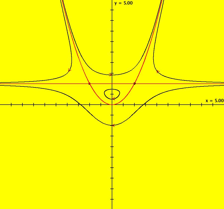
View/Sys/Gal: EMap "QuasiHamiltonian: P=y-1; Q=y-x^2" in "VectorFields." Here the generators are the parabola and the line given by: y = x^2 and y = 1 So H = P*Q where P = y-1 and Q = y-x^2. OdeFactory gives: dx/dt = (a*Q+b*P), dy/dt = -(b*(-2*x)*P) with a = b = 1. You can see that the curves defined by P = 0 and Q = 0 are solution curves even when the system is not Hamiltonian by using OdeFactory to see what happens as you vary the parameters a and b, or you can apply a bit of Math as follows: On P = 0: dx/dt = a*Py*Q and dy/dt = -(a*Px*Q) so dP/dt = Px*dx/dt+Py*dy/dt = Px*(a*Py*Q)+Py*(-(a*Px*Q)) = 0 On Q = 0: dx/dt = b*P*Qy, dy/dt = -(b*P*Qx) so dQ/dt = Qx*dx/dt+Qy*dy/dt = Qx*(b*P*Qy)+Qy*(-(b*P*Qx)) = 0 The crossing points of P = 0 and Q = 0 are fixed points for the system and the curves themselves are separatrices. When a = 0 and b ≠ 0, y = 1 turns into all fixed points. When a ≠ 0 and b = 0, y = x^2 turns into all fixed points. When a = b = 0, all points are fixed points. When the generators are linear, the global rate parameters are related to eigenvalues and eigenvectors at fixed points. See the input window called "Define an AGF" if you want to create AGFs with linear generators and/or see sections galleries "AGFExs" and "TwoComplexLines". Note: when you click "Adj Params" to play with parameters a and b, the working system changes so these comments are no longer shown. If you want to view these comments while you adjust the parameters, first select "Show All Comments" on the gallery menu then scroll to these comments. You can add your new version of the system to the current gallery, using a new name, or you can go back to the original system in the gallery, by selecting it again from the list of systems in the gallery. Image 1: Ode view. P is the red straight line, Q is the red parabola. Together they form the separatrix system for the Ode system. Image 2: The Ode R2+ view. Image 3: EMapCT9 view gives a fractal.
|
|
|
View/Sys/Gal: Ode "QuasiHamiltonian: P=y-sin(x); Q=x+sin(y)" in "VectorFields." This system of odes is defined by the equations: dx/dt = (a*Q+b*(cos(y))*P), dy/dt = -(a*(-1*cos(x))*Q+b*P) Parameters are: a = .10; b = .10; Functions are: P=y-sin(x); Q=x+sin(y) To generate the red separatrices near (0,0), zoom in several times then place the cursor near (0,0) hold the shift key down and move the cursor a bit. Then zoom back out. Image 1: Ode view with colored vector field on. Try a = 1 = -b EMapCT9 zoomed in.
|
|
|
View/Sys/Gal: EMap "QuasiHamiltonian: P=y-x^2; Q=y-c, a = -.20; b = -.84; c = -2.00; as EMapCT3" in "VectorFields." This system of odes is defined by the equations: dx/dt = (a*Q+b*P), dy/dt = -(a*(-2*x)*Q) Parameters are: c = -2.00; a = -.20; b = -.84; Functions are: P=y-x^2; Q=y-c Note that Q itself has a parameter, c. Image 1: EMapCT3 view.
|
|
|
View/Sys/Gal: Ode "QuasiHamiltonian: P=y-x^2; Q=y-c, a = 1.00; b = 1.00; c = -2.00; as Ode" in "VectorFields." This system of odes is defined by the equations: dx/dt = (a*Q+b*P), dy/dt = -(a*(-2*x)*Q) Parameters are: c = -2.00; a = 1; b = 1; Functions are: P = y-x^2; Q = y-c For this example, P and Q are solution curves but then do not form the separatrix system. Image 1: Ode view.
|
|
|
View/Sys/Gal: EMap "QuasiHamiltonian: P=y-x^2; Q=y-c, a = 1; b = 1; c = -.12; as EMap" in "VectorFields." This system of odes is defined by the equations: dx/dt = (a*Q+b*P), dy/dt = -(a*(-2*x)*Q) Parameters are: c = -.12; a = 1.00; b = 1.00; Functions are: P = y-x^2; Q = y-c Image 1: EMap view.
|
|
|
View/Sys/Gal: EMap "QuasiHamiltonian: P=y-x^2; Q=y-c, a = 1; b = 1; c = .72; as EMap" in "VectorFields." This system of odes is defined by the equations: dx/dt = (a*Q+b*P), dy/dt = -(a*(-2*x)*Q) Parameters are: c = .72; a = 1.00; b = 1.00; Functions are: P = y-x^2; Q = y-c Image 1: EMap view. This is a fractal.
|
|
|
View/Sys/Gal: EMap "QuasiHamiltonian: P=y-x^2; Q=y-c, c = -.130; a = 1.000; b = 1.300; as EMapCT2 ver 2" in "VectorFields." This iteration is defined by: x <- (a*Q+b*P), y <- -(a*(-2*x)*Q). Parameters are: c = -.130; a = 1.000; b = 1.300; Functions are: P = y-x^2; Q = y-c EMap CT: 2 Image 1: EMapCT2 view with fractal centers at about p1 = (0,0) and p2 = (.3,0). Image 2: EMapMaxCT2 view zoomed in 3X at (0.0045335,.0810427).
|
|
|
View/Sys/Gal: EMap "QuasiHamiltonian: P=y-x^2; Q=y-c, c = -.130; a = 1.000; b = 1.300; as EMapMaxCT3" in "VectorFields." This iteration is defined by: x <- (a*Q+b*P), y <- -(a*(-2*x)*Q). Parameters are: c = -.130; a = 1.000; b = 1.300; Functions are: P = y-x^2; Q = y-c EMap CT: 2 Image 1: EMapCT3 view. There are two fractal centers, one near (0,.70644) the other near (.3158,0).
|
|
|
View/Sys/Gal: Ode "QuasiHamiltonian: SHO H=y^2/(2*m)+k*x^2/2, k=1; m=1;" in "VectorFields." This is an actual Hamiltonian system from Physics. The equations are the equations of motion for a simple harmonic oscillator (mass on a spring) derived from the Hamiltonian function: (1) Enter H=y^2/(2*m)+k*x^2/2 into the "user fns:" field. (2) Enter k=1; m=1 into the "params:" field. (3) Click the "Update Sys" button. The system of odes generated by OdeFactory is: dx/dt = (a*(((2*m)*(2*y))/((2*m)^2))), dy/dt = -(a*((2*k*2*x)/4)) which simplifies to dx/dt = y/m, dy/dt = -k*x Parameters are: k=1; m=1; a = 1; Functions are: H=y^2/(2*m)+k*x^2/2 Image 1: Ode view.
|
|
|
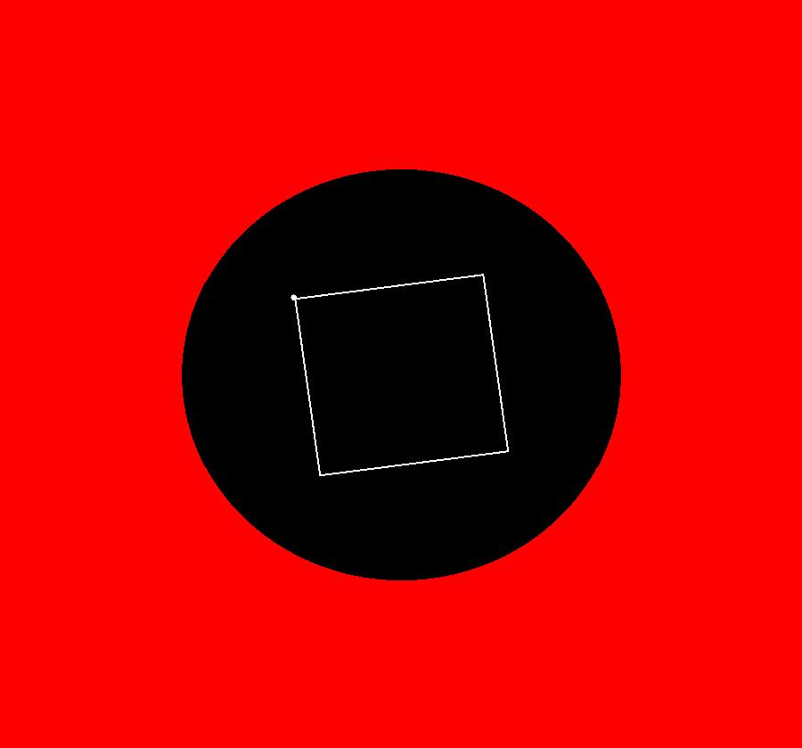
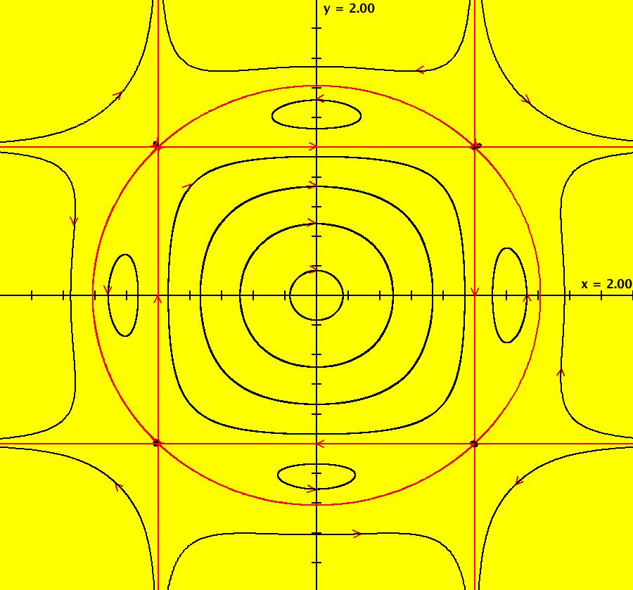
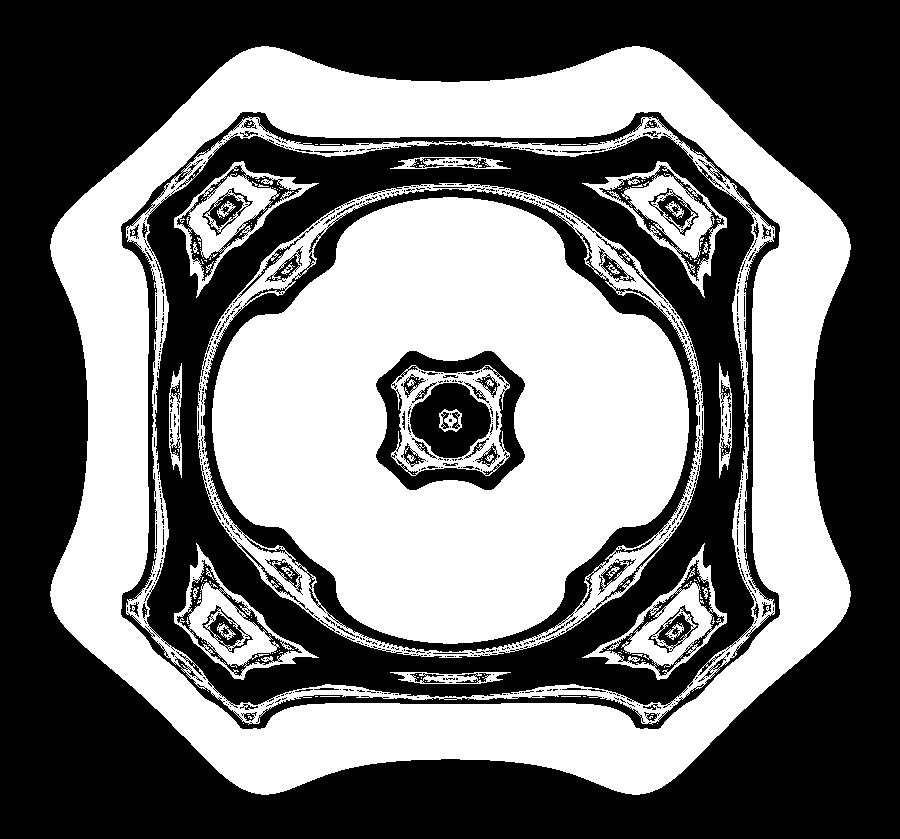
View/Sys/Gal: EMap "QuasiHamiltonian: a square in a circle" in "VectorFields." This system of odes is defined by the equations: dx/dt = (a*(2*y)*P*Q*R*S+b*H*Q*R*S+c*H*P*R*S), dy/dt = -(a*(2*x)*P*Q*R*S+d*H*P*Q*S+f*H*P*Q*R) Parameters are: a = 1; b = 1; c = 1; d = 1; f = 1; Functions are: H=x^2+y^2-2; P=y-1; Q=y+1; R=x-1; S=x+1 The square centered at (0,0) has sides of length 2 and the circle centered at (0,0) has radius sqrt(2). Image 1: Ode view. Image 2: EMapCT9 view. This is a fractal center.
|
|
|
View/Sys/Gal: EMap "QuasiHamiltonian: a square in a circle as an EMap" in "VectorFields." This iteration is defined by: x <- (a*(2*y)*P*Q*R*S+b*H*Q*R*S+c*H*P*R*S), y <- -(a*(2*x)*P*Q*R*S+d*H*P*Q*S+f*H*P*Q*R). Parameters are: a = -1.50; b = 1.00; c = 1.00; d = 1.00; f = 1.00; Functions are: H=x^2+y^2-2; P=y-1; Q=y+1; R=x-1; S=x+1 EMap CT: 0 Image 1: EMap view. This is a fractal.
|
|
|
View/Sys/Gal: Ode "QuasiHamiltonian: line, parabola, circle" in "VectorFields." This system of odes is defined by the equations: dx/dt = (a*Q*R+b*P*R+c*(2*y)*P*Q), dy/dt = -(b*(-2*x)*P*R+c*(2*x)*P*Q) Parameters are: a = 1; b = 1; c = 1; Functions are: P=y+1; Q=y-x^2; R=x^2+y^2-4 Image 1: Ode view.
|
|
|
View/Sys/Gal: EMap "QuasiHamiltonian: line, parabola, circle EMapCT5" in "VectorFields." This iteration is defined by: x <- (a*Q*R+b*P*R+c*(2*y)*P*Q), y <- -(b*(-2*x)*P*R+c*(2*x)*P*Q). Parameters are: a = 1; b = 1; c = 1; Functions are: P=y+1; Q=y-x^2; R=x^2+y^2-4 EMap CT: 5 Image 1: EMapCT5 view. Yet another fractal.
|
|
|
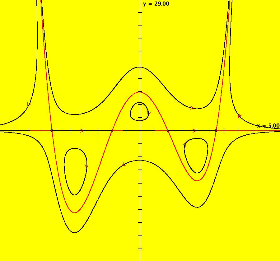
View/Sys/Gal: Ode "QuasiHamiltonian: solving (x^2-1)*(x-e)*(x+pi)=0" in "VectorFields." The zeros of the function f(x) are at the intersection of the curves y = f(x) and y = 0. To find these points, using OdeFactory, define a quasiHamiltonian system using F = y-f(x), G = y and find the fixed points of the system that are on both y = f(x) and y = 0. For example, if f(x)=(x^2-1)*(x-e)*(x+pi), then F=y-(x^2-1)*(x-e)*(x+pi), G=y
and the system of odes is defined by the equations: dx/dt = (c*G+d*F), dy/dt = -(c*(-1*(x^2-1)*(x-e)-(x^2-1+(2*x)*(x-e))*(x+pi))*G). Parameters are: a = 1; b = 1; c = 1; d = 1; To find the zeros of f(x), turn the colored vector field on then zoom in on each fixed point. To see y = f(x), draw the separatrix system. OdeFactory gives fixed points on both y = f(x) and y = 0 at: x = -3.141595, -1.000002, 1.000007, 2.718281. Notice that a quasiHamiltonian system of odes always has fixed points at the crossing points of the generating functions, F(x,y) and G(x,y), and that it can have fixed points that are not on the generating functions. The latter are called spontaneous critical points. Another (perhaps faster and better) way to find, or verify, the zeros of f(x) is to start two trajectories on y = 0 and examine their +t and -t limits by clicking on the starting points. Starting trajectories at (2,0) and (-2,0) gives: x = -3.141593, -1.000000, 1.000000, 2.718282. Image 1: Ode view.
|
|
|
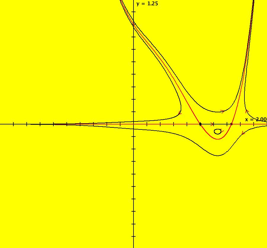
View/Sys/Gal: Ode "QuasiHamiltonian: solving 1-x+x^2-2*x^3+x^4=0" in "VectorFields." This system of odes is defined by the equations: dx/dt = (a*G+b*F), dy/dt = -(a*(-2*x+1+6*x^2-4*x^3)*G). Parameters are: a = 1; b = 1; Functions are: F=y-(1-x+x^2-2*x^3+x^4); G=y Zeros of y = 1-x+x^2-2*x^3+x^4 are at x = 0.999930, 1.465718 Starting a trajectory at (1.2,0) gives x = 1.000000, 1.465571. Image 1: Ode view.
|
|
|
View/Sys/Gal: EMap "QuasiHamiltonian: square" in "VectorFields." This system of odes is defined by the equations: dx/dt = (a*Q*R*S+b*P*R*S), dy/dt = -(c*P*Q*S+d*P*Q*R) Parameters are: a = 1; b = 1; c = 1; d = 1; Functions are: P=y-1; Q=y+1; R=x-1; S=x+1 Image 1: Ode view. Image 2: EMapCT9 view.
|
|
|
View/Sys/Gal: Ode "QuasiHamiltonian: two crossing circles" in "VectorFields." This system of odes is defined by the equations: dx/dt = (a*(2*y)*Q+b*(2*y)*P), dy/dt = -(a*(2*x-2)*Q+b*(2*x+2)*P) Parameters are: a = 1; b = 1; Functions are: P=(x-1)^2+y^2-4; Q=(x+1)^2+y^2-4 Image 1: Ode view.
|
|
An OdeFactory Slide Show Click on a slide to zoom in. Click "video" to see a video. |
View/Sys/Gal: Ode "TwoComplexLines: ***** Introduction *****" in "VectorFields." ***** Introduction ***** These are some examples from a book I wrote in 1973 called "Algebraically Generated Flows." I used the systems in this section to verify that OdeFactory gives the same results that I calculated by hand in 1973. The twelve systems are keyed to figures in the book. Select item "AGFs" on the Help menu to see an online copy of the book.
|
|
|
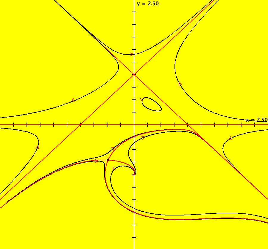
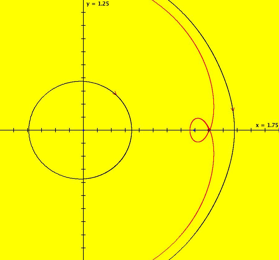
View/Sys/Gal: Ode "TwoComplexLines: fig 5.2.1: a = 2, w2 = 1, x* = 1/3" in "VectorFields." This AGF is generated by the lines: I[1]: x+i*y = 0, λ = i I[2]: (x-1)+0.5*i*y = 0, λ = i The degree of the RHS of the system is: 3. A spontaneous critical point is at: x* = 1/(1+a) where a = Im(lambda)/abs(Im(b)) so a = 2 => Im(b) = .5 Image 1: Ode view.
|
|
|
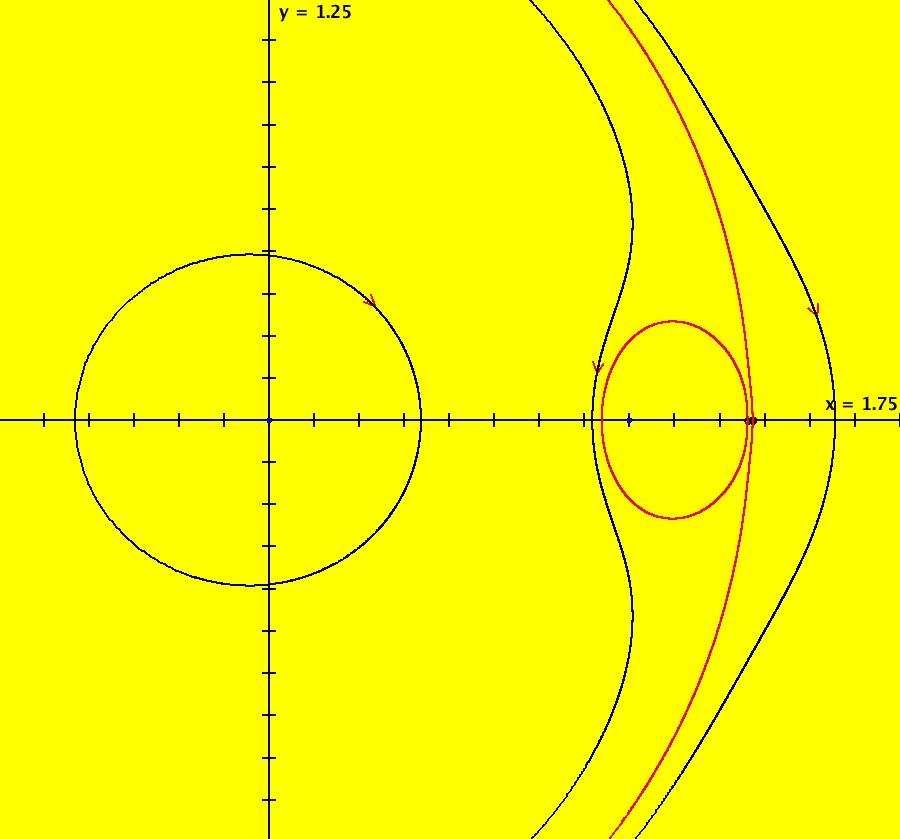
View/Sys/Gal: Ode "TwoComplexLines: fig 5.2.2: a = 0, w2 = 0, x* = 1" in "VectorFields." This AGF is generated by the lines: I[1]: x+i*y = 0, λ = i I[2]: (x-1)+0.5*i*y = 0, λ = 0 The degree of the RHS of the system is: 3. Image 1: Ode view.
|
|
|
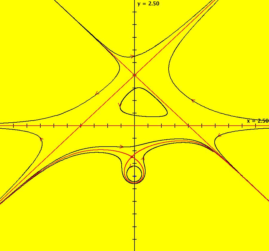
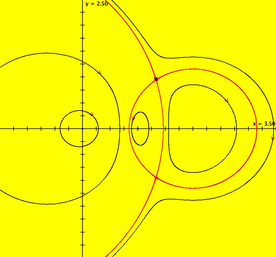
View/Sys/Gal: Ode "TwoComplexLines: fig 5.2.3: a = -1/8, w2 = -1/16, x* = 8/7" in "VectorFields." This AGF is generated by the lines: I[1]: x+i*y = 0, λ = i I[2]: (x-0.99)+0.5*i*y = 0, λ = -0.0625*i The degree of the RHS of the system is: 3. This AGF is generated by the lines: I[1]: x+i*y = 0, λ = i I[2]: (x-0.99)+0.5*i*y = 0, λ = -0.0625*i The degree of the RHS of the system is: 3. Image 1: Ode view.
|
|
|
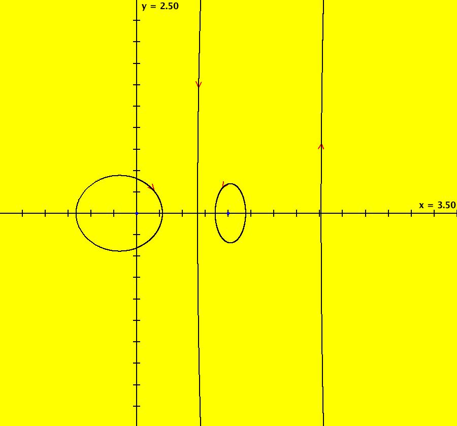
View/Sys/Gal: Ode "TwoComplexLines: fig 5.2.4: a = -1/4, w2 = -1/8, x* = 4/3" in "VectorFields." This AGF is generated by the lines: I[1]: x+i*y = 0, λ = i I[2]: (x-1)+0.5*i*y = 0, λ = -0.125*i The degree of the RHS of the system is: 3. Image 1: Ode view.
|
|
|
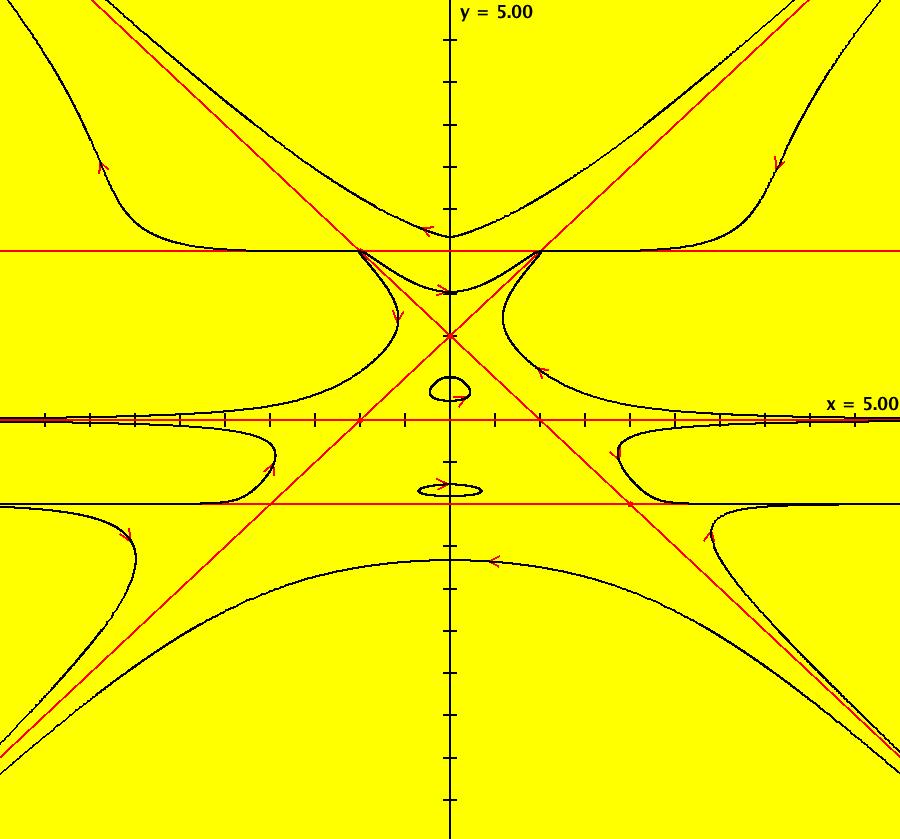
View/Sys/Gal: Ode "TwoComplexLines: fig 5.2.5: a = -1/2, w2 = -1/4, x* = 2" in "VectorFields." This AGF is generated by the lines: I[1]: x+i*y = 0, λ = i I[2]: (x-1)+0.5*i*y = 0, λ = -0.25*i The degree of the RHS of the system is: 3. Image 1: Ode view.
|
|
|
View/Sys/Gal: Ode "TwoComplexLines: fig 5.2.6: a = -1, w2 = -1/2 no x*" in "VectorFields." This AGF is generated by the lines: I[1]: x+i*y = 0, λ = i I[2]: (x-1)+0.5*i*y = 0, λ = -0.5*i The degree of the RHS of the system is: 3. Image 1: Ode view.
|
|
|
View/Sys/Gal: EMap "TwoComplexLines: fig 5.2.6: view as an EMapMaxCT3 variation" in "VectorFields." This AGF is generated by the lines: I[1]: x+i*y = 0, λ = i I[2]: 1.4*(x-1)+0.5*i*y = 0, λ = -0.5*i The degree of the RHS of the system is: 3. Image 1: EMapMaxCT3 view.
|
|
|
View/Sys/Gal: EMap "TwoComplexLines: fig 5.2.6: w/Re(a) for I[2]) = 1.4 EMapMaxCT3" in "VectorFields." This AGF is generated by the lines: I[1]: x+i*y = 0, λ1 = i I[2]: 1.4*(x-1)+0.5*i*y = 0, λ2 = -0.5*i The degree of the RHS of the system is: 3. Image 1: EMapMaxCT3 view.
|
|
|
View/Sys/Gal: Ode "TwoComplexLines: fig 5.3: fig 5.2.1 with Re(b2) > 0" in "VectorFields." This AGF is generated by the lines: I[1]: x+i*y = 0, λ = i I[2]: (x-1)+(0.5+0.5*i)*y = 0, λ = i The degree of the RHS of the system is: 3. Image 1: Ode view.
|
|
|
View/Sys/Gal: Ode "TwoComplexLines: fig 5.4: fig 5.2.1 with Re(═) = .1" in "VectorFields." This AGF is generated by the lines: I[1]: x+i*y = 0, λ = i I[2]: (x-1)+(0.5+0.5*i)*y = 0, λ = (0.1+i) The degree of the RHS of the system is: 3. Image 1: Ode view.
|
|
|
View/Sys/Gal: Ode "TwoComplexLines: fig 5.5 as AGF" in "VectorFields." This AGF is generated by the lines: I[1]: x+i*y = 0, λ = 0 I[2]: (x-1)+(0.5+0.5*i)*y = 0, λ = 1 The degree of the RHS of the system is: 3. Image 1: Ode R2+ view.
|
|
|
View/Sys/Gal: Ode "TwoComplexLines: fig 5.5 from dx/dt and dy/dt" in "VectorFields." This system of odes is defined by the system: dx/dt = (x-1)*P, dy/dt = y*P Functions are: P = x^2+y^2 Image 1: Ode view.
|