Click on an image to go directly to a system or scroll to see the systems in this gallery.
 |
 |
 |
 |
 |
 |
 |
 |
 |
 |
 |
 |
 |
 |
 |
 |
 |
 |
 |
 |
 |
 |
 |
 |
 |
 |
| OdeFactory Images and Annotations | |
|
An OdeFactory Slide Show Click on a slide to zoom in. Click "video" to see a video. |
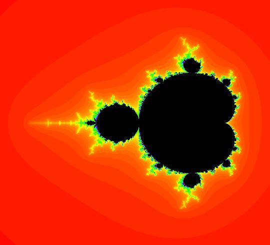
View/Sys/Gal: Ode " AGFs and Mandelbrot Julia Sets" in "AGFs&Mandelbrot." AGFs and Mandelbrot Julia Sets This gallery demonstrates how to generate the Mandelbrot Julia sets associated with the quadratic iteration z <- z^2+c using AGFs. It also shows how to get from the Mandelbrot Julia sets to related cubic iterations via an AGF. The Mandelbrot iteration is z <- z^2+c, where z and c are complex, or x <- x^2-y^2+p, y <- 2*x*y+q where x, y, p and q are real. Note that if the system of odes has a fixed point at (a,b) then (-a,-b) is also a fixed point. The Jacobian of the system is: J = {{2x,-2y},{2y,2x}} so J(-a,-b) = -J(a,b) and the eigenvalues at the two fixed points just differ by a sign. Consequently, every Mandelbrot Julia set for the iteration z <- z^2+c can be generated from an AGF defined as follows: (1) given p and q, use WA to solve x^2-y^2+p = 0, 2*x*y+q = 0 for the fixed points (a,b) and (-a,-b). (2) apply WA to evaluate D[{x^2-y^2,2*x*y},{{x,y}}] at x=a, y=b to find λ (3) define the AGF using two complex lines: I[1]: (x-a)+i*(y-b), λ1 = λ and I[2]: (x+a)+i*(y+b), λ2 = - λ To investigate cubic iterations related to the Mandelbrot JSets, create an AGF using the algorithm shown above then open parameter controllers for the two complex generators and vary some of the 16 control parameters. See system (6) for example. To view the Julia sets use the EMap (escape time) view in OdeFactory. To get the Mandelbrot set from the AGF, use WA to find the "dx/dt, dy/dt" form of the AGF then add p to the dx/dt equation and q to the dy/dt equation and create the companion 4D system. In the (x,y) view, set (x,y,z,w) = (0,0,0,0) then go to the EMap view.
|
|
|
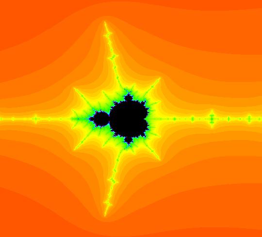
View/Sys/Gal: EMap "(1a) (x^2-y^2+p,2*x*y+q), p = -1.00; q = .00" in "AGFs&Mandelbrot." This system of odes is defined by the equations: dx/dt = x^2-y^2+p, dy/dt = 2*x*y+q Parameters are: p = -1.00; q = .00; Setting x^2-y^2-1=0 and 2*x*y=0 gives fixed points at (-1,0) and (1,0). J = {{2*x,-2*y},{2*y,2*x}} J(-1,0) = {{-2,0},{0,-2}}, λ = -2 J(1,0) = {{2,0},{0,2}}, λ = 2 Using I[1]: (x+1)+i*y, λ1 = -2 and I[2]: (x-1)+i*y, λ2 = 2 gives system (2). Try the EMap view w/various color tables. Try changing parameter values.
|
|
|
View/Sys/Gal: EMap "(1b) MSet of (1a), (x,y,z^2-w^2+x,2*z*w+y) EMap" in "AGFs&Mandelbrot." This system of odes is defined by the equations: dx/dt = x, dy/dt = y, dz/dt = z^2-w^2+x, dw/dt = 2*z*w+y. It comes from the Mandelbrot iteration: "z <- z^2+c" or dx/dt = x^2-y^2+p, dy/dt = 2*x&y+q via the 4d companion system.
|
|
|
View/Sys/Gal: EMap "(1c) another view of (1b) EMapCT6" in "AGFs&Mandelbrot." This system of odes is defined by the equations: dx/dt = x, dy/dt = y, dz/dt = z^2-w^2+x, dw/dt = 2*z*w+y. Zoom out to see where this on the Mandelbrot set.
|
|
|
View/Sys/Gal: EMap "(1d) variation of (1c), (x,y,0.5*(1-z^2+w^2)+x,-z*w+y) EMapCT6" in "AGFs&Mandelbrot." This system of odes is defined by the equations: dx/dt = x, dy/dt = y, dz/dt = 0.5*(1-z^2+w^2)+x, dw/dt = -z*w+y.
|
|
|
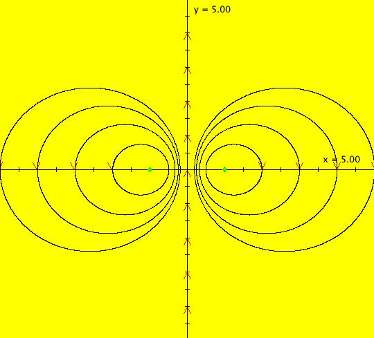
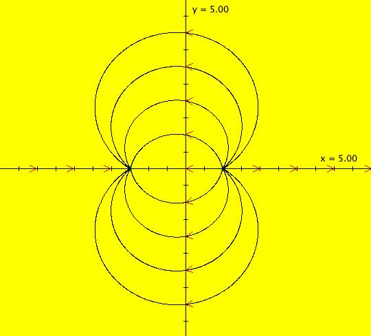
View/Sys/Gal: Ode "(2a) AGF: star-in & star-out, same as system (1a)" in "AGFs&Mandelbrot." This is called the potential flow from a doublet or a doblet flow. It is the superposition of a source, at (1,0), and a sink, at (-1,0), with the same strength. This AGF is generated by the lines: I[1]: (x+1)+i*y = 0, λ = -2 I[2]: (x-1)+i*y = 0, λ = 2 A general AGF generated by 2 complex generators has degree 3 but symmetry reduces the degree of this particular system to 2. The "dx/dt, dy/dt" equations corresponding to the AGF are: dx/dt = ((-1.000*(x+1.000))*((0.500*(x-1.000)^2)+(0.500*(y)^2))+(1.000*(x-1.000))*((0.500*(x+1.000)^2)+(0.500*(y)^2))), dy/dt = -(((1.000*(y))*((0.500*(x-1.000)^2)+(0.500*(y)^2))+(-1.000*(y))*((0.500*(x+1.000)^2)+(0.500*(y)^2)))). which simplify to dx/dt = x^2-y^2-1, dy/dt = 2*x*y. as expected. Another way to see that system (1) and (2) are the same is to note that the vector fields are the same when you toggle between the two systems. What happens to the EMap when you change the: (a) locations of the fixed points while preserving the symmetry (a,b) and (-a,-b) and keeping the λs constant? (b) locations of the fixed points without preserving the symmetry (a,b) and (-a,-b) but still keeping the λs constant? (c) λs while keeping the fixed points constant and preserving the symmetry λ2 = - λ1? (d) λs while keeping the fixed points constant but not preserving the symmetry λ2 = - λ1? You can answer these questions by opening text-based parameter controllers for the two AGF generators by clicking on the green dots while in the Ode view. Then get into the EMap view, change the parameters and see what happens.
|
|
|
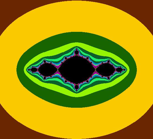
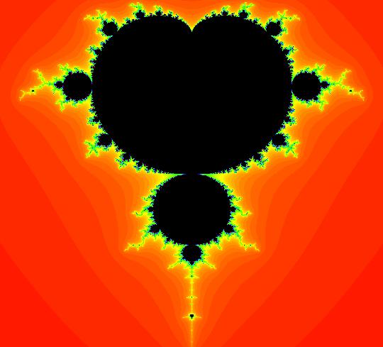
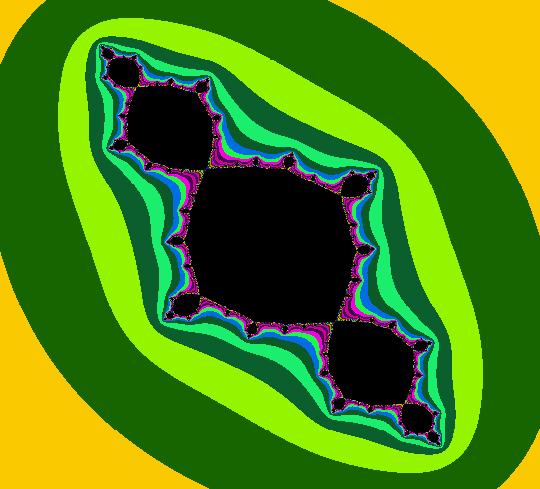
View/Sys/Gal: EMap "(2b) MSet of (2a), EMap (x,y,z^2-w^2-1+x,2*z*w+y)" in "AGFs&Mandelbrot." This system of odes is defined by the equations: dx/dt = x, dy/dt = y, dz/dt = z^2-w^2-1+x, dw/dt = 2*z*w+y. View the small black region on the left.
|
|
|
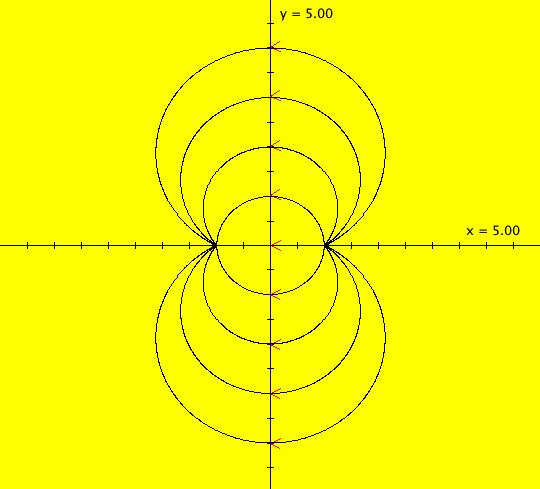
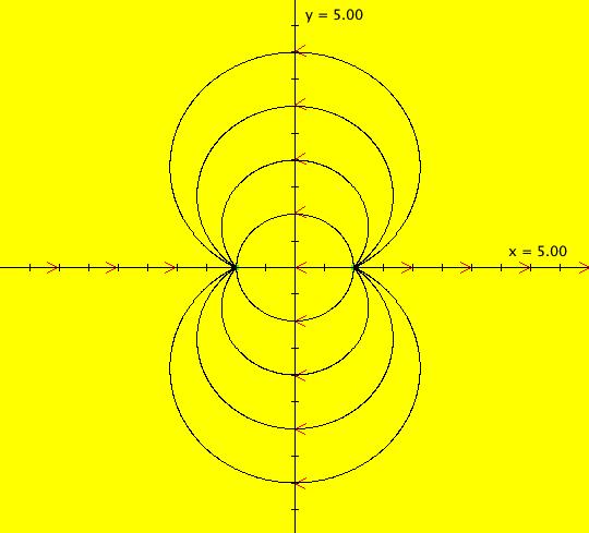
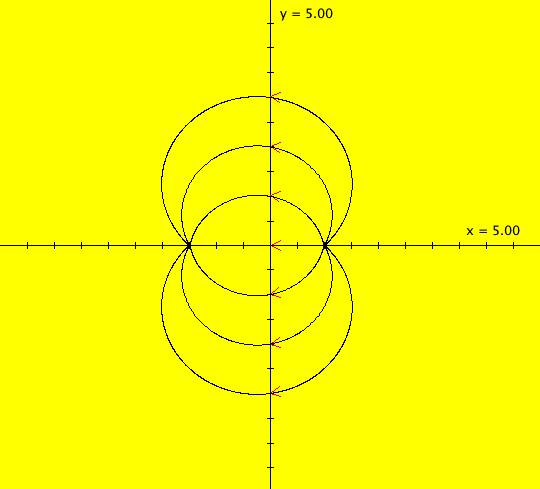
View/Sys/Gal: Ode "(3a) AGF: perpendicular to star in, star out" in "AGFs&Mandelbrot." These are the equi-potential lines for the doublet flow. They are orthogonal to the doublet flow trajectories. This AGF is generated by the lines: I[1]: (x+1)+i*y = 0, λ1 = -2*i I[2]: (x-1)+i*y = 0, λ2 = 2*i The degree of the RHS of the system is: 3. dx/dt = ((-1.000*(y))*((0.500*(x-1.000)^2)+(0.500*(y)^2))+(1.000*(y))*((0.500*(x+1.000)^2)+(0.500*(y)^2))) dy/dt = -(((-1.000*(x+1.000))*((0.500*(x-1.000)^2)+(0.500*(y)^2))+(1.000*(x-1.000))*((0.500*(x+1.000)^2)+(0.500*(y)^2)))) which simplify to dx/dt = 2*x*y, dy/dt = -(x^2-y^2-1).
|
|
|
View/Sys/Gal: EMap "(3b) MSet of (3a), EMap (x,y,2*z*w+x,-(z^2-w^2-1)+y)" in "AGFs&Mandelbrot." This system of odes is defined by the equations: dx/dt = x, dy/dt = y, dz/dt = 2*z*w+x, dw/dt = -(z^2-w^2-1)+y.
|
|
|
View/Sys/Gal: EMap "(4a) AGF: star-in & star-out, fixed points moved, as EMap" in "AGFs&Mandelbrot." This AGF is generated by the lines: I[1]: (x+0.4851)+i*(y-0.62874) = 0, λ = -2 I[2]: (x-0.4851)+i*(y+0.62874) = 0, λ = 2 The degree of the RHS of the system is generally 3 but it is 2 in this case because of symmetry. dx/dt = -0.485268+0.76921*x^2 -1.99519*x*y-0.76921*y^2, dy/dt = 0.629348+0.997594*x^2 +1.53842*x*y-0.997594*y^2.
|
|
|
View/Sys/Gal: EMap "(4b) MSet of (4a), EMap (x,y,-0.485268+0.76921*z^2-1.99519*z*w-0.76921*w^2+x,0.629348+0.997594*z^2+1.53842*z*w-0.997594*w^2+y)" in "AGFs&Mandelbrot." This system of odes is defined by the equations: dx/dt = x, dy/dt = y, dz/dt = -0.485268+0.76921*z^2 -1.99519*z*w-0.76921*w^2+x, dw/dt = 0.629348+0.997594*z^2 +1.53842*z*w-0.997594*w^2+y.
|
|
|
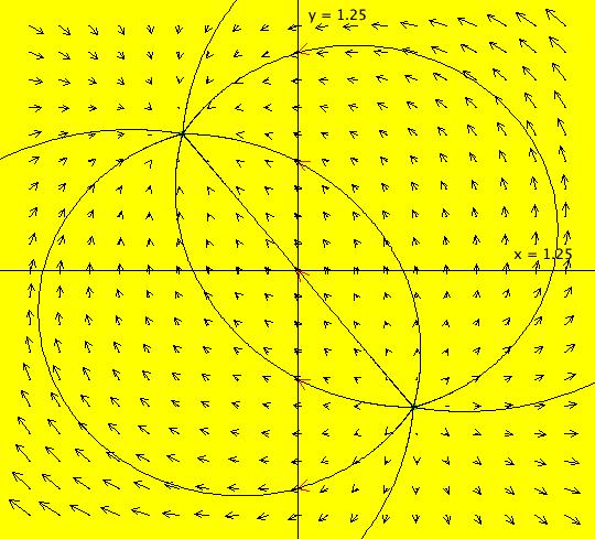
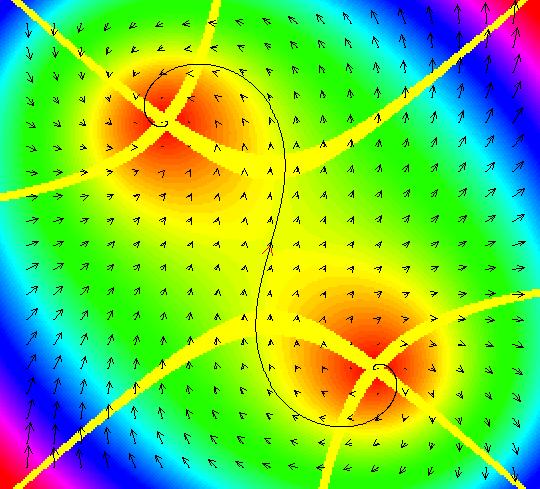
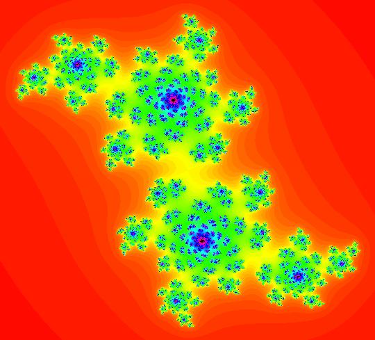
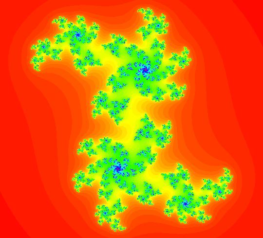
View/Sys/Gal: EMap "(5a) (x^2-y^2+p,2*x*y+q), p = .16; q = .61; as EMap" in "AGFs&Mandelbrot." The colored vector field shows the fixed points where the (yellow) nullclines cross. The EMap view shows the Julia set for (p,q) = (.16,.61). The red dot is the start of the orbit at (0,0). The orbit escapes. In the Ode view, if you open an editor for the trajectory at (0,0) you will find that the fixed points are at +-(-.485095,.628743). Use WA on evaluate D[{x^2-y^2+.16,2*x*y+.61},{{x,y}}] at x=-.485095, y=.628743 to find the eigenvalues at the fixed points: λ = +-(-.97019-1.25749*i) The next system, (5b),was created by using these fixed points and eigenvalues for the complex generators.
|
|
|
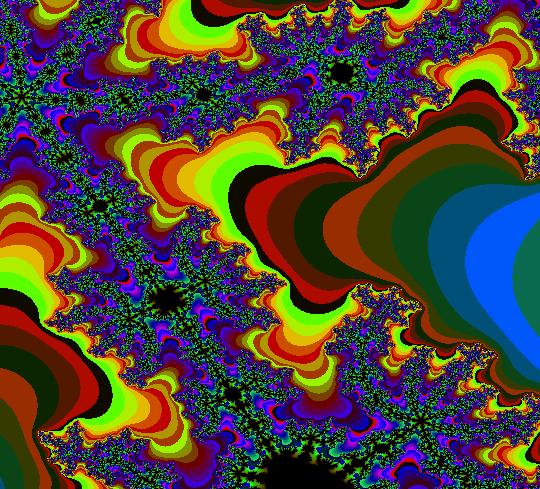
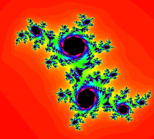
View/Sys/Gal: EMap "(5b) AGF: spiral-in & spiral-out, fixed points moved, as EMap" in "AGFs&Mandelbrot." This AGF is generated by the lines: I[1]: (x+0.49)+i*(y-0.63) = 0, λ = (-0.97019-1.25749*i) I[2]: (x-0.49)+i*(y+0.63) = 0, λ = (0.97019+1.25749*i) The degree of the RHS of the system is generally 3 but it is 2 in this case because of symmetry. dx/dt = 0.15825+ 0.99519*x^2+0.00714*x*y-0.99519 *y^2 dy/dt = 0.613871- 0.00357*x^2+1.99038*x*y+0.00357*y^2 Does the location of I[1], at the fixed point point (x,y) = (-.49,.63), in the Ode view, have any particular significance in the EMap view? To answer this question center at the point, get into the EMap view then zoom in several times.
|
|
|
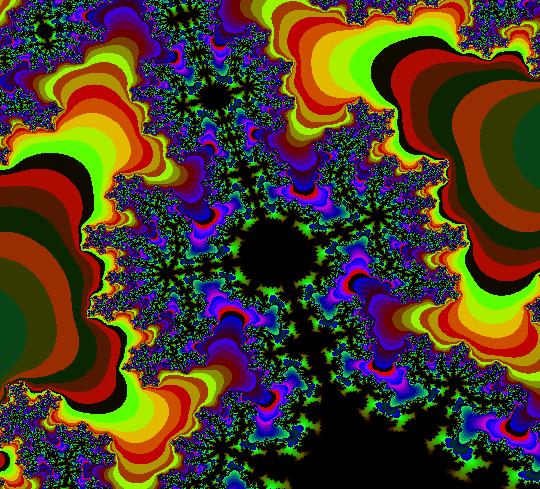
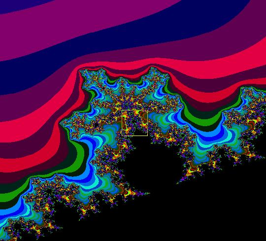
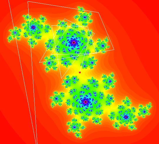
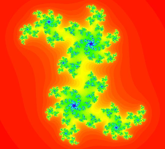
View/Sys/Gal: EMap "(6) AGF: spiral-in & spiral-out, fixed points moved, ver 2 as EMap" in "AGFs&Mandelbrot." This AGF is generated by the lines: I[1]: (1-0.02*i)*(x+0.45)+(0.04+1.1*i)*(y-0.64) = 0, λ = (-0.97-1.3*i) I[2]: (1.1-0.03*i)*(x-0.51)+(-0.04+1.1*i)*(y+0.69) = 0, λ = (0.81+1.3*i) In this case the symmetry of the vector field is lost. The EMap looks similar to a Julia set associated with the Mandelbrot iteration, z <- z^2+c but it is not a Mandelbrot Julia set. To zoom in at a point in the EMap view, ctrl-drag at the point to open a selection circle then click the "Update" button in the "Graphics Settings" window. To return to the original view of the system, open it again using the selection list.
|
|
|
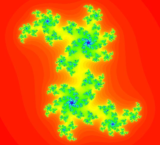
View/Sys/Gal: EMap "(7a) (x^2-y^2+p,2*x*y+q), p = .380; q = .380; as EMap" in "AGFs&Mandelbrot." The Mandelbrot iteration is defined by: x <- x^2-y^2+p, y <- 2*x*y+q. Parameters are: p = .380; q = .380; To find the fixed points open a trajectory editor to get: p(100.000000) = (-0.280536,0.677274) p(0.000000) = (0.000000,-1.000000) p(-100.000000) = (0.280536,-0.677274) so the fixed points are: (x1,y1) = (-.280536,.677274) and (x2,y2) = (.280536,-.677274). Then apply WA to the Jacobian at the fixed points evaluate D[{x^2-y^2+.38,2*x*y+.38},{{x,y}}] at x=-.280536, y=.677274 to get λ1 = -.561072+-i*1.35455 and λ2 = .561072+-i*1.35455
|
|
|
View/Sys/Gal: EMap "(7b) AGF: ccw spiral in & cw spiral out, as EMap" in "AGFs&Mandelbrot." This AGF is generated by the lines: I[1]: (x+0.280536)+i*(y-0.677274) = 0, λ1 = (-0.561072-1.35455*i) I[2]: (x-0.280536)+i*(y+0.677274) = 0, λ2 = (0.561072+1.35455*i) The degree of the RHS of the system would normally be 3 but it reduces to 2 because of symmetry.
|
|
|
View/Sys/Gal: EMap "(7c) dx/dt. dy/dt version of (7b), as an EMap" in "AGFs&Mandelbrot." This system of odes is defined by the equations: dx/dt = ((-0.522*(x+0.281)-1.260*(y-0.677))*((0.500*(x-0.281)^2)+(0.500*(y+0.677)^2))+(0.522*(x-0.281)+1.260*(y+0.677))*((0.500*(x+0.281)^2)+(0.500*(y-0.677)^2))), dy/dt = -(((-1.260*(x+0.281)+0.522*(y-0.677))*((0.500*(x-0.281)^2)+(0.500*(y+0.677)^2))+(1.260*(x-0.281)-0.522*(y+0.677))*((0.500*(x+0.281)^2)+(0.500*(y-0.677)^2)))) . Using this three digit precision expanded polynomial form of the AGF generated vector field is a less efficient (slower) way to compute the image. It gives fair agreement with (7a) and (7b) in the Ode and EMap views but to get agreement in the IMap view full 16 digit precision constants need to be used.
|
|
|
View/Sys/Gal: EMap "(8a) AGF: not symmetric" in "AGFs&Mandelbrot." This AGF is generated by the lines: I[1]: (x+1.5)+i*y = 0, λ1 = -2 I[2]: (x-1)+i*y = 0, λ2 = 2 Or dx/dt = ((-0.640*(x+1.500))*((0.500*(x-1.000)^2)+(0.500*(y)^2))+(0.640*(x-1.000))*((0.500*(x+1.500)^2)+(0.500*(y)^2))) = -1.2+(0.4+0.8*x)*x-0.8*y^2, dy/dt = -(((0.640*(y))*((0.500*(x-1.000)^2)+(0.500*(y)^2))+(-0.640*(y))*((0.500*(x+1.500)^2)+(0.500*(y)^2)))) = 0.4*y+1.6*x*y
|
|
|
View/Sys/Gal: EMap "(8b) AGF: in dx/dt. dy.dt form, not symmetric" in "AGFs&Mandelbrot." This system of odes is defined by the equations: dx/dt = -1.2+(0.4+0.8*x)*x-0.8*y^2, dy/dt = 0.4*y+1.6*x*y.
|
|
|
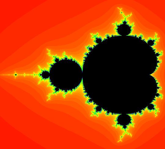
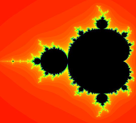
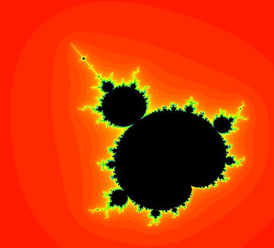
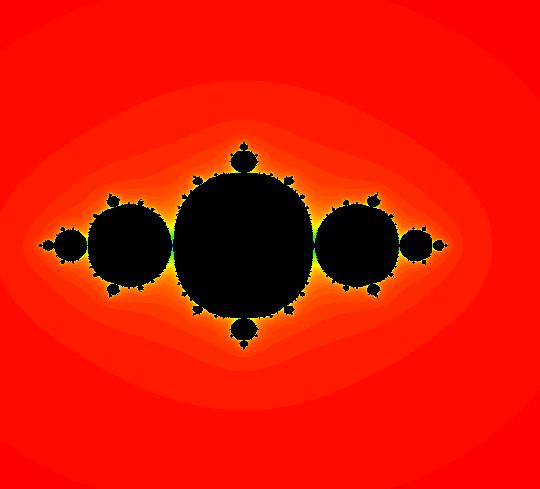
View/Sys/Gal: EMap "(8c) bifurcation diagram of (8b) EMap" in "AGFs&Mandelbrot." This system of odes is defined by the equations: dx/dt = x, dy/dt = y, dz/dt = -1.2+(0.4+0.8*z)*z-0.8*w^2+x, dw/dt = 0.4*w+1.6*z*w+y. It is the bifurcation diagram of system (8b) and it is a distortion of the Mandelbrot set.
|