Click on an image to go directly to a system or scroll to see the systems in this gallery.
 |
|
 |
 |
 |
 |
 |
 |
 |
 |
 |
 |
 |
 |
 |
 |
 |
 |
 |
 |
 |
 |
 |
 |
 |
 |
 |
 |
 |
 |
 |
 |
 |
 |
 |
 |
 |
 |
 |
 |
 |
 |
 |
 |
 |
 |
 |
 |
 |
 |
 |
 |
 |
 |
 |
 |
 |
 |
 |
 |
 |
 |
 |
 |
 |
 |
 |
 |
 |
 |
 |
 |
 |
 |
 |
 |
 |
 |
 |
 |
 |
 |
 |
 |
 |
 |
 |
 |
 |
 |
 |
 |
 |
 |
 |
 |
 |
 |
 |
 |
 |
 |
 |
 |
 |
 |
 |
 |
 |
 |
 |
 |
 |
 |
 |
 |
 |
 |
 |
 |
 |
 |
 |
 |
 |
 |
 |
 |
 |
 |
 |
 |
 |
 |
 |
 |
 |
 |
 |
| OdeFactory Images and Annotations | |
|
|
View/Sys/Gal: IMap "1D: IMap (x^2+c), c = -1.00; " in "MapExs." From Hubbard and West, "Differential Equations: A Dynamical Systems Approach Part I," p. 201, 5.1.2.
This iteration is defined by:
x <- x^2+c.
Parameters are:
c = -1.00;
ICs: (x,t) = (-1,0) so,
x0 = -1, x1 = 0, x2 = -1, ... or
xn = ((-1)^(n+1)-1)/2
Adjust c.
Try: c = -1.3 and c = -1.8
|
|
|
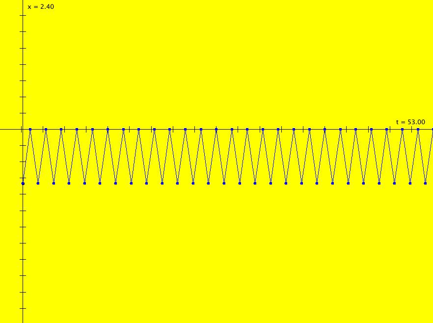
View/Sys/Gal: IMap "1D: IMap x <- (3.5+b*.1)*x*(1-x), logistic map" in "MapExs." Generally the logistic map is written as:
x <- r*x*(1-x),
where r is the bifurcation parameter. I want to look at values of r near 3.5 so I rewrote r as (3.5+b*.1).
This iteration is defined by:
x <- (3.5+b*.1)*x*(1-x).
Parameters are:
b = -1.00;
A trajectory/orbit has been started at (0,0.5).
In the IMap view slowly increase b and watch what happens. Whenever the dots line up in horizontal rows (your eye will spot this condition), the number of rows of dots will be the period of the periodic orbit.
To observe chaotic behavior due to slightly different starting values, start a second orbit at (0,.501) then adjust b = 2.5.
See the next system "logistic bifurcation map."
|
|
|
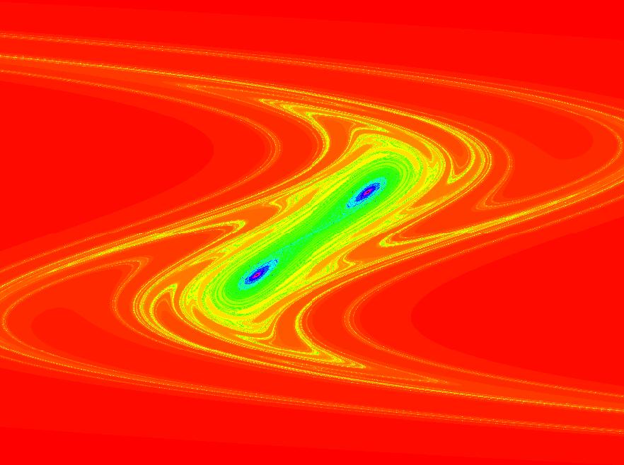
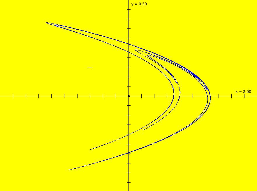
View/Sys/Gal: EMap "2D: Duffing map, EMap view" in "MapExs." This iteration is defined by:
x <- y,
y <- -b*x+a*y-y^3.
Parameters are:
a = 2.30; b = 1.10;
Also try the Ode view.
|
|
|
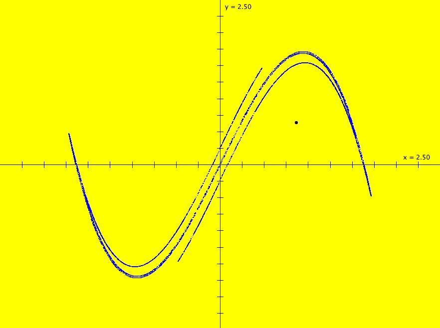
View/Sys/Gal: IMap "2D: Duffing map, IMap view" in "MapExs." This iteration is defined by:
x <- = y,
y <- -b*x+a*y-y^3.
Parameters are:
a=2.75; b=.15
The black dot is the seed. Do an animation to see how the iteration works.
For a list of interesting iterative maps see: chaotic maps>.
|
|
|
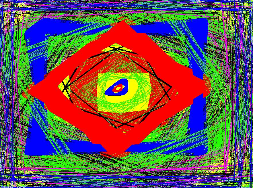
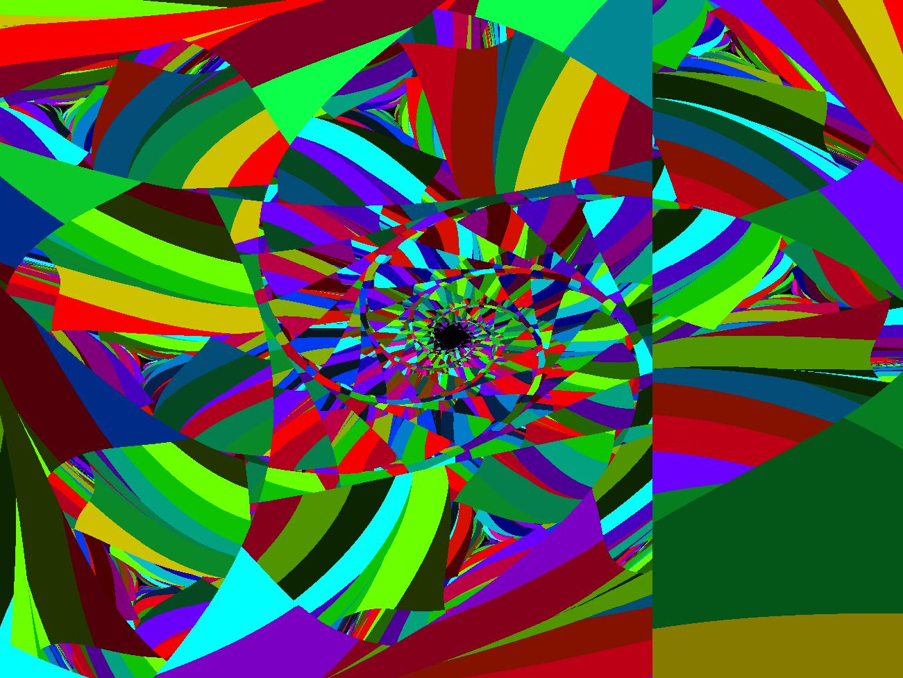
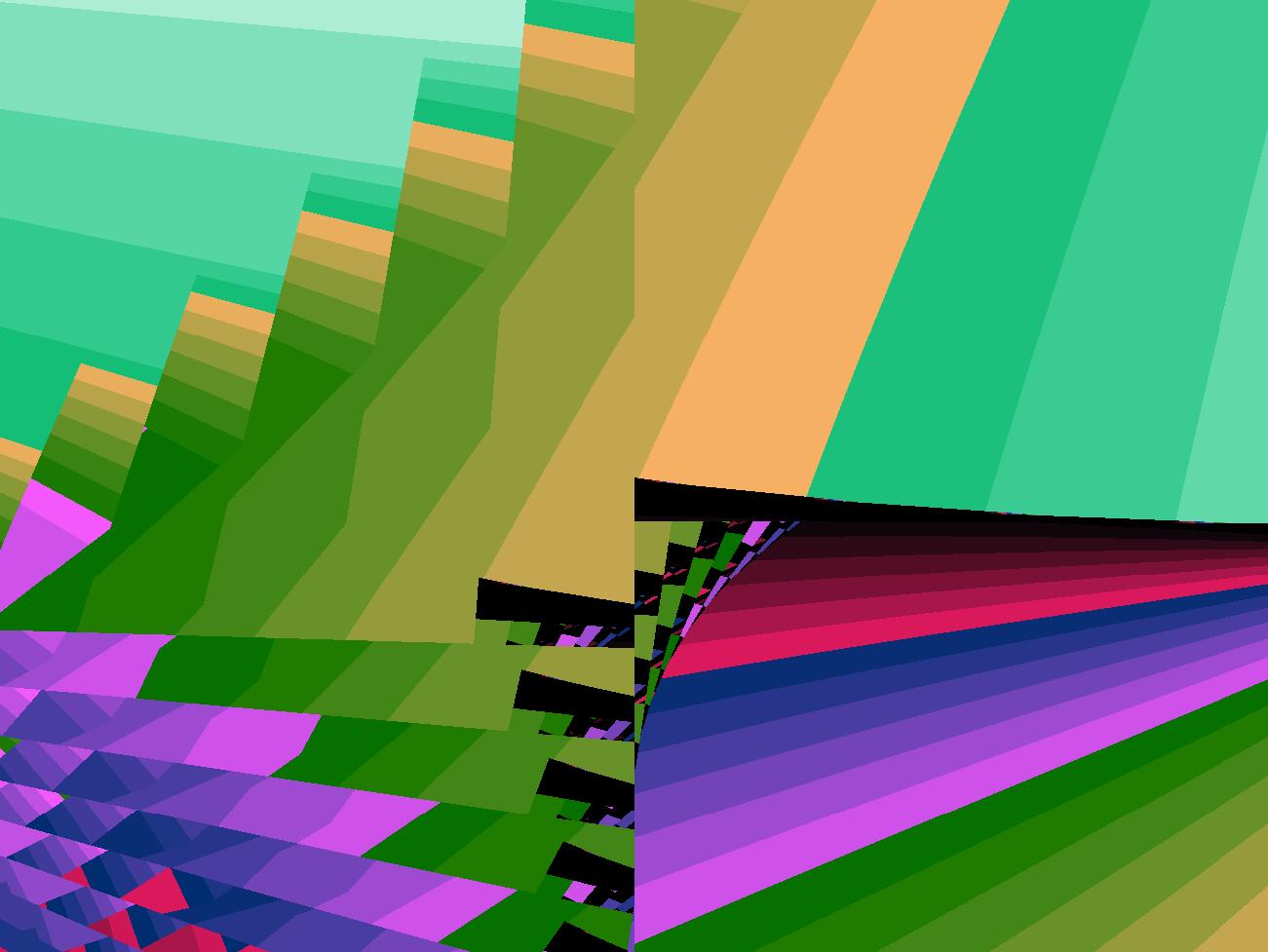
View/Sys/Gal: EMap "2D: EMap Barry Martin map #2, variation 3" in "MapExs." This iteration is defined by:
x <- y-abs(x)/x*sqrt(abs(b*x-c)),
y <- a-x.
Parameters are:
a = -2.40; b = -.20; c = 3.80;
Zoom out to see what this image is part of.
|
|
|
View/Sys/Gal: EMap "2D: EMap Barry Martin map #2, variation 4" in "MapExs." This iteration is defined by:
x <- (1+s*.01)*(y-abs(x)/x*sqrt(abs(b*x-c))),
y <- (1+s*.01)*(a-x).
Parameters are:
a = -2.40; b = -.20; c = 3.80; s=0
This is part of image:
2D: EMap Barry Martin map #2, variation 3
with a time scaling factor.
Try adjusting s and the other parameters.
|
|
|
View/Sys/Gal: EMap "2D: EMap Barry Martin map #2, variation 4, CT demo" in "MapExs." This iteration is defined by:
x <- (1+s*.01)*(y-abs(x)/x*sqrt(abs(b*x-c))),
y <- (1+s*.01)*(a-x).
Parameters are:
a = -.700; b = .280; c = 4.600; s = 2.600;
Click in the graphics area to open the color table controller then try the various color tables.
|
|
|
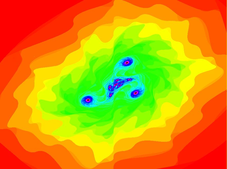
View/Sys/Gal: EMap "2D: EMap Barry Martin map #2, variation 4, Three body problem." in "MapExs." This iteration is defined by:
x <- (1+.1*s)*(y-abs(x)/x*sqrt(abs(b*x-c))),
y <- (1+.1*s)*(a-x).
Parameters are:
a = .500; b = 1.000; c = .000; s = .450;
Try some other color tables.
|
|
|
View/Sys/Gal: EMap "2D: EMap Chirikov map" in "MapExs." This iteration is defined by:
x <- (1+s*.01)*((x-k*sin(y))%6.283),
y <- (1+s*.01)*((y+x)%6.283).
Parameters are:
k = .90; s = .60;
|
|
|
View/Sys/Gal: EMap "2D: EMap Gingerbreadman map, variation 1" in "MapExs." This iteration is defined by:
x <- 1-y+abs(x),
y <- x%a.
Parameters are:
a = 1.50;
This vector field is generally shown in the IMap view.
Try some other color tables.
|
|
|
View/Sys/Gal: EMap "2D: EMap Gingerbreadman map, variation 2a" in "MapExs." This iteration is defined by:
x <- 1-y+abs(x)%b,
y <- x%a.
Parameters are:
a = 9.00; b = 4.20;
|
|
|
View/Sys/Gal: EMap "2D: EMap Gingerbreadman map, variation 2b" in "MapExs." This system is:
x <- 1-y+abs(x)%b,
y <- x%a.
Parameters are:
a = 5.20; b = 6.10;
The Gingerbreadman is beginning to appear.
|
|
|
View/Sys/Gal: EMap "2D: EMap Gingerbreadman map, variation 3" in "MapExs." This iteration is defined by:
x <- (1+s*.01)*(1-y+abs(x)%b),
y <- (1+s*.01)*x%a.
Parameters are:
a = 9.50; b = -5.80; s = 1.90;
The factor (1+s*.01) scales time.
|
|
|
View/Sys/Gal: EMap "2D: EMap Henon map ver 2" in "MapExs." The iteration is defined by:
x <- (1+s*.01)*(1-a*x^2+y),
y <- (1+s*.01)*b*y
Parameters are:
a = .52; b = 1.00; s = 3.00;
Try the various color tables.
|
|
|
View/Sys/Gal: EMap "2D: EMap Henon map ver 3" in "MapExs." The iteration is defined by:
x <- 1-a*x^2+y,
y <- (1+b*.01)*x.
Parameters are:
a = .20; b = 1
Also see: Henon map
|
|
|
View/Sys/Gal: EMap "2D: EMap Henon map ver 4" in "MapExs." This iteration is defined by:
x <- 1-a*x^2+y,
y <- (1+b*.01)*x.
Parameters are:
a = .10; b = 2.60;
Zoom out to see what this image is part of.
|
|
|
View/Sys/Gal: EMap "2D: EMap Henon map ver 5" in "MapExs." This iteration is defined by:
x <- y+1-a*x^2,
y <- b*x.
Parameters are:
a = .200; b = 1.100;
|
|
|
View/Sys/Gal: EMap "2D: EMap Henon map ver 6" in "MapExs." This iteration is defined by:
x <- 1-a*x^2+y,
y <- (1+b*.01)*x.
Parameters are:
a = .520; b = 3.700;
Use EMap CT: 3
|
|
|
View/Sys/Gal: EMap "2D: EMap Henon quadratic twist map, ver 2" in "MapExs." This iteration is defined by:
x <- x*cos(a)-(y-x^2)*sin(a),
y <- x*sin(a)+(y-x^2)*cos(a).
Parameters are:
a = 4.00;
|
|
|
View/Sys/Gal: EMap "2D: EMap Hubbard & West example, p. 87" in "MapExs." The system is:
x <- F,
y <- y+.7*F*(1-F^2/25),
Functions are:
F=x+.7*y
Also try the IMap view. Try various ICs by clicking in the viewing area.
For more details, see: "MacMath" by Hubbard and West, 1992, p. 87-90.
|
|
|
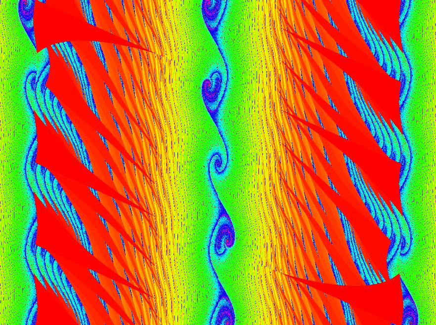
View/Sys/Gal: EMap "2D: EMap Standard map" in "MapExs." The system is time-scaled.
This iteration is defined by:
x <- (1+s*.01)*((x-k*sin(y))%6.283),
y <- (1+s*.01)*((y+x)%6.283).
Parameters are:
k = .07; s = 6.20;
|
|
|
View/Sys/Gal: EMap "2D: EMap Standard map, ver 2" in "MapExs." This iteration is defined by:
x <- (1+s*.01)*(x+y-k/6.283*sin(6.283*x)),
y <- (1+s*.01)*(y-k/6.283*sin(6.283*x)).
Parameters are:
k = 1.70; s = 1.40;
|
|
|
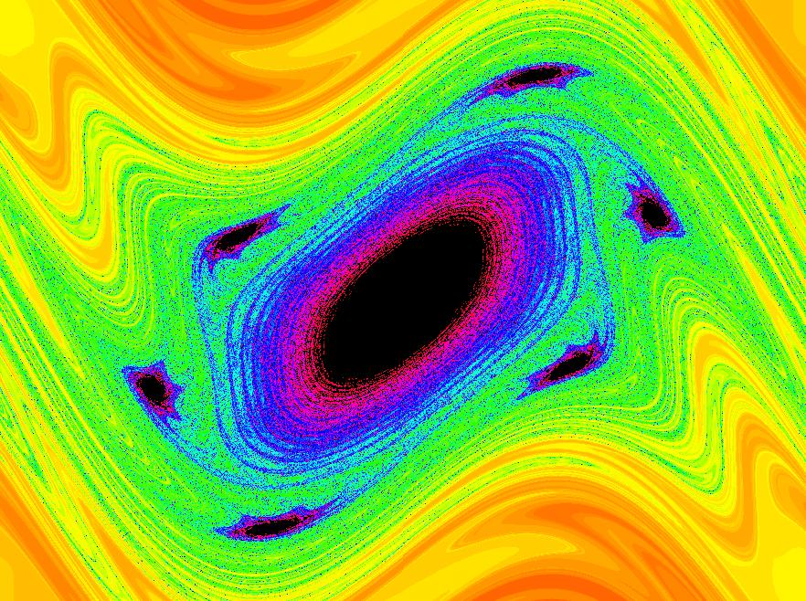
View/Sys/Gal: EMap "2D: EMap pendulum as a fractal" in "MapExs." This iteration is defined by:
x <- y,
y <- -k*sin(x)-c*y+d*sin(a*t).
Parameters are:
k = 5.800; c = .000; d = -.260; a = .300;
We seem to have some quasi-periodic trajectories in the Ode view, bounded chaotic orbits in the IMap view and fractals in the EMap view.
This is color table 5. Try some other color tables.
|
|
|
View/Sys/Gal: IMap "2D: IMap Barry Martin map #1" in "MapExs." This iteration is defined by:
x <- y-sin(x),
y <- a-x.
Parameters are: a = 1.00;
The black dots are the seed values.
Toggle "Show 2D IMap Orbit Sequence" on the Help menu. Notice the difference.
Toggle "Hide Axes" on the Help menu. Notice the difference.
Toggle "Hide Arrowheads/Seeds" on the Help menu. Notice the difference.
Play with the parameter "a".
To see how the map works, click the "Clear" button while in the IMap view then click in the graphics area to start an orbit. Click again to start more orbits.
Also check out the EMap view.
The system originated with Barry Martin of Birmingham England and it is cited in "MacMath" by Hubbard and West, p. 92, 1992.
See also: demos of the Martin map.
Here are some references from the above web site:
"The Martin map equations were taken from:
M. Trott, The Mathematica GuideBook for Programming, New York: Springer-Verlag, 2004 pp. 347�349.
B. Martin, "Graphic Potential of Recursive Functions," J. Landsdown, R. A. Earnshaw, eds., Computers in Art, Design and Animation, New York: Springer�Verlag, 1989 pp. 109�129.
The Martin Map is also called the "Hopalong-Attractor".
See also: Hopalong Image Generator and a German website: Huepfer.
|
|
|
View/Sys/Gal: IMap "2D: IMap Barry Martin map #1, variation 1" in "MapExs." This iteration is defined by:
x <- y-sqrt(abs(x)),
y <- a-x.
Parameters are:
a = 1.00;
Also try the EMap view.
|
|
|
View/Sys/Gal: IMap "2D: IMap Barry Martin map #1, variation 2" in "MapExs." This iteration is defined by:
x <- y-abs(x)/x*sqrt(abs(b*x-c)),
y <- a-x.
Parameters are:
a = 1.00; b=1; c=1
Also try the EMap view.
See: Wolfram demos
|
|
|
View/Sys/Gal: IMap "2D: IMap Barry Martin map #2" in "MapExs." This system is:
x <- y-abs(x)/x*sqrt(abs(b*x-c)),
y <- a-x.
Parameters are:
a=.5; b=1; c=0
The abs(x)/x could be replaced by sgn(x).
There is a period-17 orbit at seed
(x,y) = (-3.294575,-2.650030).
To see the orbit, start a Flow animation. Notice that the animation visits the 17 small islands. You can also see the orbit by selecting "Show 2D IMap Orbit Sequence" on the Help menu. Also, try turning on "Show Approximate IMap Orbit Period" on the Help menu.
|
|
|
View/Sys/Gal: EMap "2D: IMap Barry Martin map #2, variation 1" in "MapExs." This system is:
x <- y-abs(x)/x*cos(abs(b*x-c)),
y <- a-x.
Parameters are:
a=.5; b=1; c=0
Also try the EMap view.
The Ode view shows the non-smoothness of the system.
Turn the colored vector field on.
NOTE: abs(x)/x can be replaced by sgn(x) and cos(abs(f(x))) can be replaced by cos(f(x)).
|
|
|
View/Sys/Gal: IMap "2D: IMap Barry Martin map #2, variation 2" in "MapExs." This system is:
x <- y-abs(x)/x*sin(abs(b*x-c)),
y <- a-x.
Parameters are:
a=.5; b=1; c=0
NOTE: abs(x)/x can be replaced by sgn(x).
|
|
|
View/Sys/Gal: IMap "2D: IMap Barry Martin map #2, variation 3" in "MapExs." This iteration is defined by:
x <- y-sgn(x)*sqrt(abs(b*x-c)),
y <- a-x.
Parameters are:
a = .54; b = .43; c = .84;
Zoom in to see more detail near the origin. Zoom back out.
Toggle "Show 2D IMap Orbit Sequence."
The parameter values have been chosen at random to give an interesting IMap.
Play with the parameters.
Also play with the system in the EMap view.
You can get back to the original state by selecting the system again. You can save an interesting new version of the system by selecting "Add to Gallery" on the OdeSystem menu.
To increase the scale on any of the sliders, move the slider to the edge of the range then close and reopen the parameter controller.
To decrease the scale on any of the sliders (to get finer control of the slider position), move the slider to the center of the range then close and reopen the parameter controller.
If you want to create your own version of the IMap, get into the IMap view then clear the existing orbits using the "Clear" button. Next add starting points (new seeds). The new orbits in the IMap view will not get their new colors until you force a redraw. Clicking the "Center" button is an easy way to force a redraw.
|
|
|
View/Sys/Gal: IMap "2D: IMap Gingerbreadman map" in "MapExs." This system is:
x <- 1-y+abs(x),
y <- x.
In the IMap view,
(1,1) is a fixed point and
(3,-1) is a 5-cycle.
Try adding some control parameters.
Try the EMap view.
|
|
|
View/Sys/Gal: IMap "2D: IMap Henon map" in "MapExs." This system is:
x <- y+1-a*x^2,
y <- b*x.
Start a flow.
See: Henon system.
|
|
|
View/Sys/Gal: IMap "2D: IMap Hubbard & West example, p. 22" in "MapExs." This system is:
x <- x^2-y,
y <- x.
For more details, see: "MacMath" by Hubbard and West, 1992, p. 22-24.
|
|
|
View/Sys/Gal: IMap "2D: IMap Hubbard & West example, p. 87, w/param" in "MapExs." This system is:
x <- F,
y <- y+.7*F*(1-a*F^2/25).
Parameters are:
a = .90;
Functions are:
F=x+.7*y
This is a variation of H&W, p.87 example with a control parameter "a" added. In the original version, "a" was 1. In this version you can adjust "a" to see what happens,
Have fun!
|
|
|
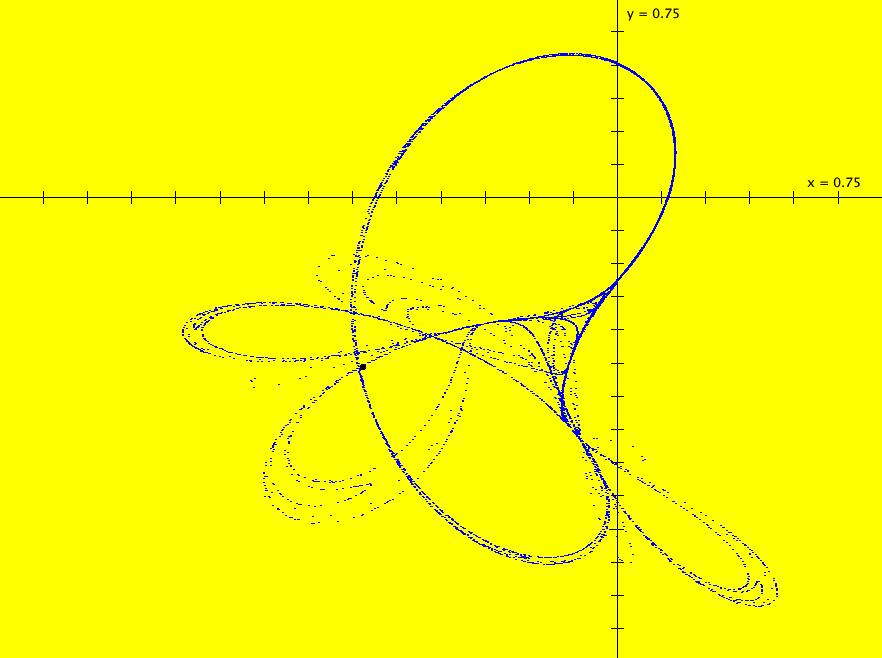
View/Sys/Gal: IMap "2D: IMap Tinkerbell map" in "MapExs." This system is:
x <- x^2-y^2+a*x+b*y,
y <- 2*x*y+c*x+d*y.
Parameters are:
a=.9; b=-.6013; c=2; d=.5
The seed is the black dot at:
(x0,y0) = (-.72,-.64).
See if you can find an interesting EMap by adjusting the parameters.
|
|
|
View/Sys/Gal: IMap "2D: IMap pendulum" in "MapExs." The system is:
x <- y,
y <- -k*sin(x)-c*y+d*sin(a*t).
Parameters are:
k=1.2; c=.3; d=.8; a=.2
The seed is at (1,0).
Vary the parameters in the IMap view.
Also try the Ode view.
As an ode - every trajectory goes to a periodic solution (but not to the same periodic solution). One way to see this is to start a flow with: 50 random dots, max speed and a 30 second duration.
See the gallery PendulumExs.
|
|
|
View/Sys/Gal: IMap "2D: IMap0011 Henon quadratic twist map (aka KAM Torus)" in "MapExs." This system is:
x <- x*cos(a)-(y-x^2)*sin(a),
y <- x*sin(a)+(y-x^2)*cos(a).
Parameters are:
a=1.3
Also see: KAM Torus and KAM: Automatic Planning and Interpretation of Numerical Experiments Using Geometrical Methods.
Try a = -1.3.
Turn "Show 2D IMap Orbit Sequence" on then vary "a" near 3.1.
|
|
|
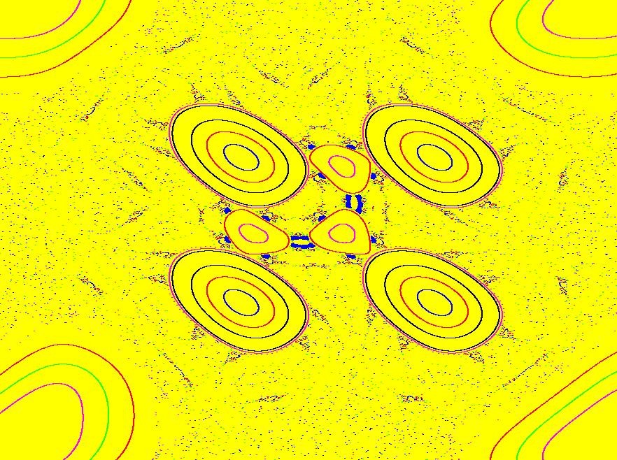
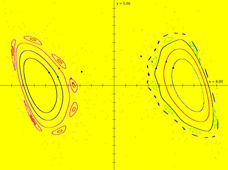
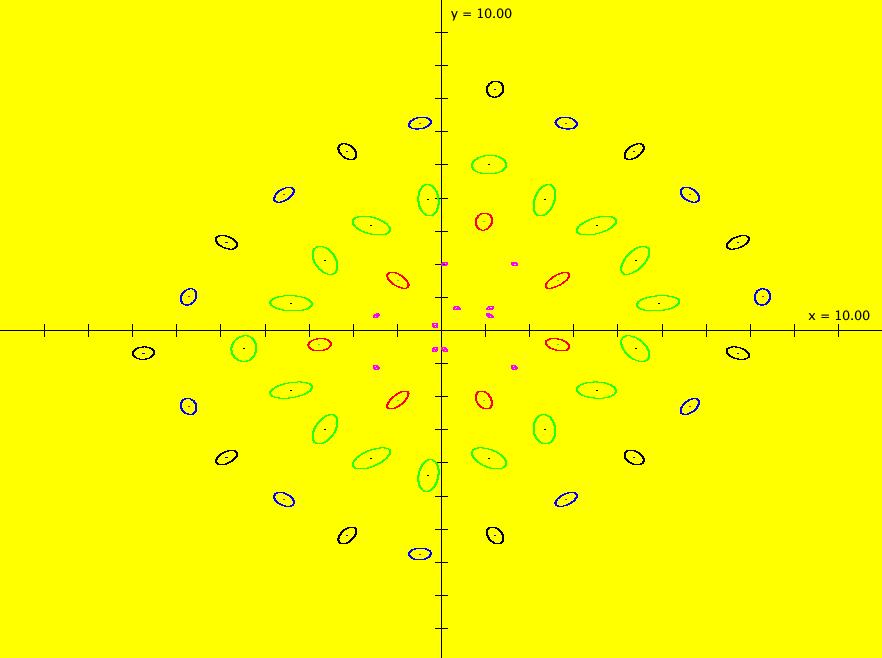
View/Sys/Gal: IMap "2D: IMap0101 Barry Martin map #2, variation 4" in "MapExs." This iteration is defined by:
x <- y-sgn(x)*sqrt(abs(b*x-c)),
y <- a-x.
Parameters are:
a = .54; b = .43; c = .84;
These are KAM island chains. The "center" of an island in an n island is a seed for an orbit of period n.
For example, there is a black orbit, of period 18, at
(x,y) = (-3.411038,0.836097),
in the center of the green 18-island chain.
If you select "Show 2D IMap Orbit Sequence" on, on the Help menu, you will see the orbit. Or - you could simply run a Flow animation.
|
|
|
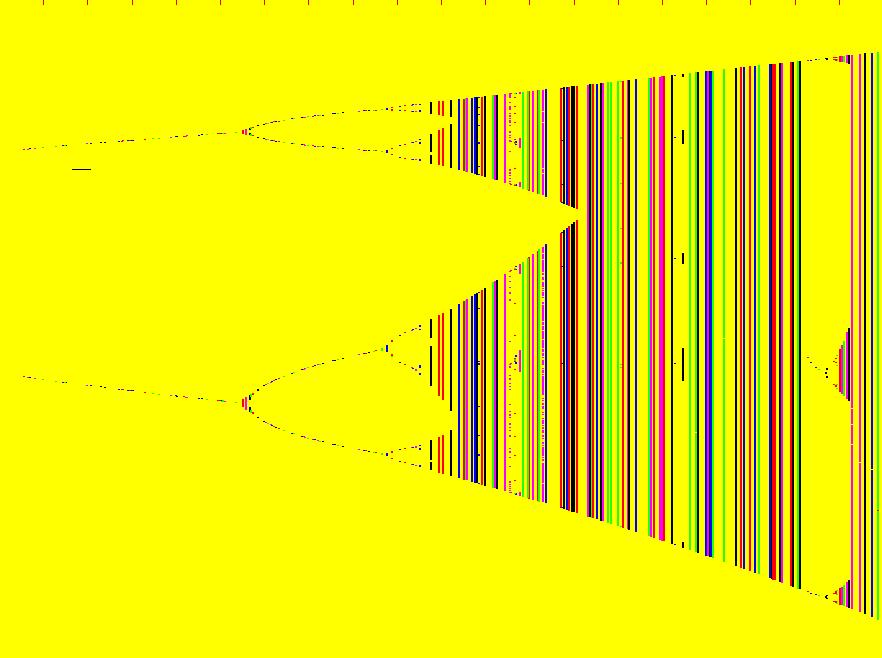
View/Sys/Gal: IMap "2D: IMap0101 x <- x, y <- x*y*(y-1), logistic bifurcation map" in "MapExs." This is the bifurcation diagram of the 1D logistic map
x <- b*x*(1-x),
where b is the bifurcation parameter.
The diagram is generated by first replacing x by y and then rewriting the 1D iteration as
y <- b*y*(1-y).
Next replace the bifurcation parameter b by the variable x and consider the 2D system:
x <- x, (x now plays the role of b)
y <- x*y*(1-y) (the original 1D map)
The IMap view of the 2D system shows the orbits of the 1D system as dots projected onto the vertical lines x = b.
See "Nonlinear Dynamics and Chaos," by Steven Strogatz p. 357 fig 10.2.7 for more details.
To generate the bifurcation diagram, start several orbits in the IMap view.
Vertical lines with n dots are period-n orbits of the 1D system. Solid vertical lines are chaotic orbits of the 1D system.
To view an orbit of period 2, clear the IMap view then start an orbit at (3.4,.5) and run a flow animation. You will see red dots accumulating on the line x = 3.4 at about y = .447 and y = .839. Another way to view this orbit is to change hMax to 100 and go to the 3D/(t,y) view to see the time-series for the orbit.
If you go back to system
"1D: IMap x <- (3.5+b*.1)*x*(1-x), logistic map"
you will see that the min and max on the x(t) curve are at about x = .447 and x = .839.
The extra dots on the x = 3.4 line when you run the flow animation in the 2D IMap view are the first few iteration points. You don't see them in the 1D example since the t axis is from 248 to 500, i.e. the transient part of the iteration is not shown.
Starting on the left, the open "windows" in the bifurcation show the period-doubling of the periodic orbits. Click in the windows to start a new and see its period.
|
|
|
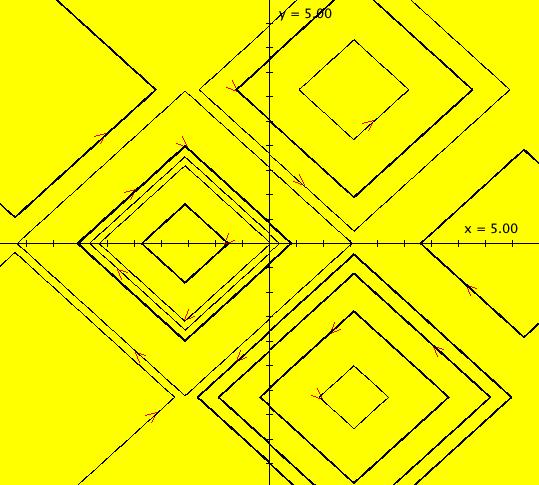
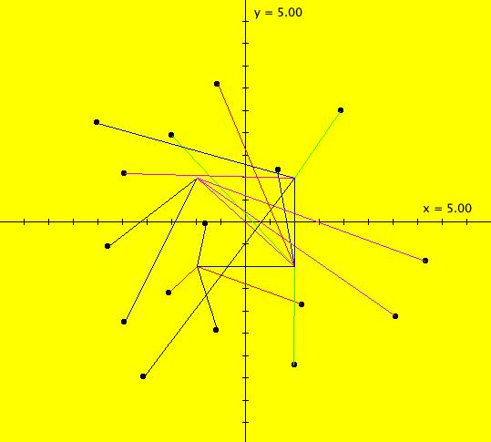
View/Sys/Gal: IMap "2D: IMap1000 (sgn(sin(y)),-sgn(cos(x))) square cycles as Ode" in "MapExs." This system of odes is defined by the equations:
dx/dt = sgn(sin(y)),
dy/dt = -sgn(cos(x)).
When viewed as an IMap, every orbit goes to (x,y) = (-1,-1).
When viewed as an Ode, this system has square cycles. |
|
|
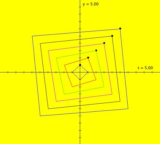
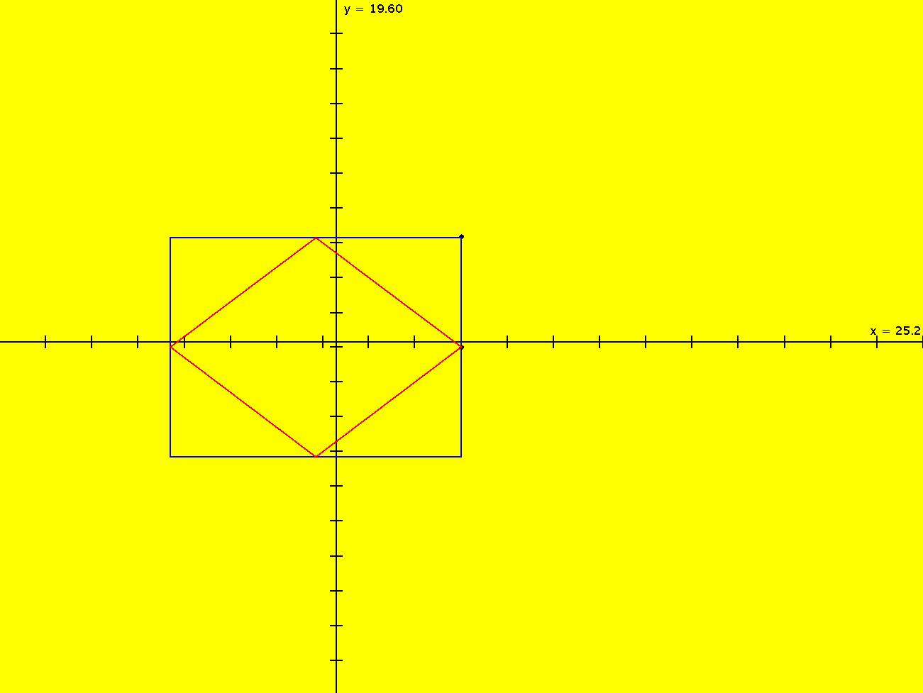
View/Sys/Gal: Ode "2D: IMap1000 (y,-x) squaring circles" in "MapExs." This iteration is defined by:
x <- y, y <- -x.
Every orbit is a 4-cycle where the points define a square. To prove this, notice that:
p0 = (x,y) -> p1 = (y,-x) -> p2 = (-x,-y) -> p3 = (-y,x) -> p4 = (x,y)
To show that the 4 points define a square, compute the length of the diagonals. The distance from p0 to p2 is x^2+y^2 and the distance from p1 to p3 is y^2+(-x)^2.
In the Ode view we get circles.
|
|
|
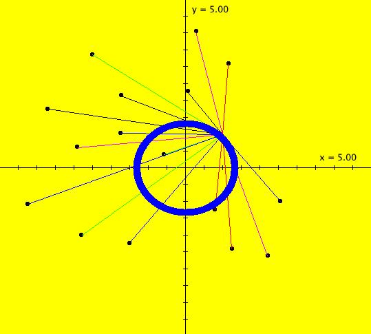
View/Sys/Gal: IMap "2D: IMap1000 circles map revisited" in "MapExs." In the Ode view, the system
dx/dt = y, dy/dt = -x
defines a family of circles about the origin. The general solution is
(x,y) = (a*sin(t)+b*cos(t),a*cos(t)-b*sin(t)).
which is another vector field that can be used to define a new 2D system of odes or a an iteration map
x <- a*sin(t)+b*cos(t),
y <- a*cos(t)-b*sin(t).
The orbits of the iteration map, after the 1st iteration, are a circle of radius
r = sqrt(a^2+b^2).
To see the circle, deselect "Show 2D IMap Orbit Sequence."
|
|
|
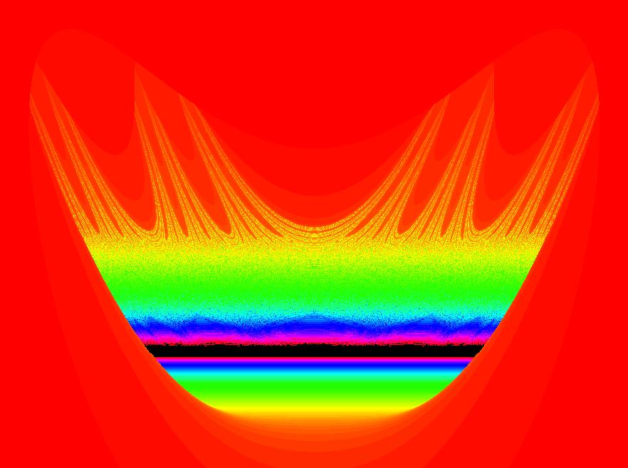
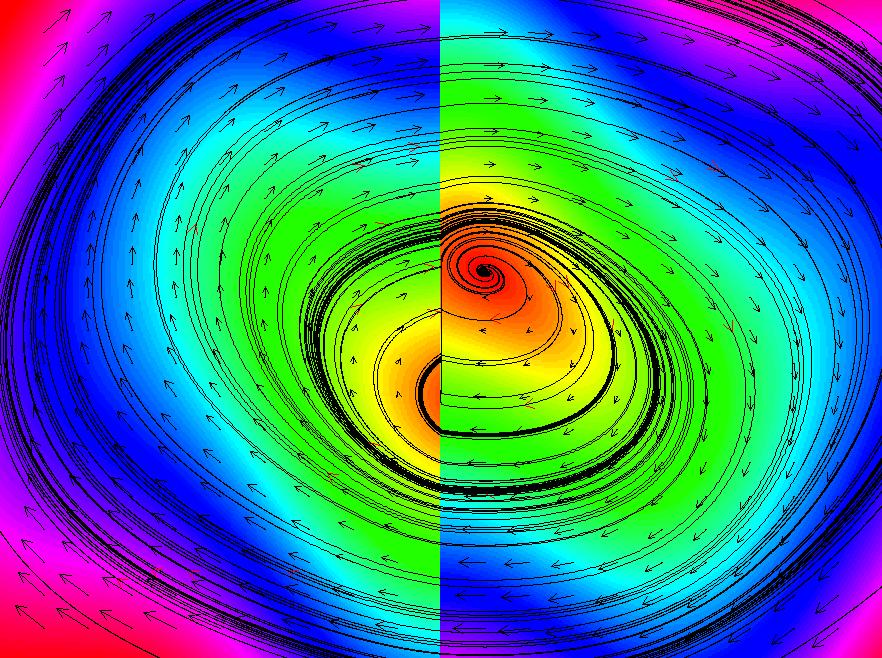
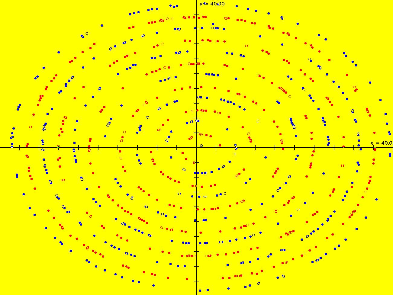
View/Sys/Gal: Ode "2D: Ode/imap/emap" in "MapExs." This system of odes is defined by the equations:
dx/dt = y-cos(x),
dy/dt = a-x.
Parameters are:
a = 1.00;
It is interesting in the Ode view, the IMap view and the EMap view.
In the Ode view, search for limit cycles using a Monte Carlo method.
Note: you need a fast machine for this method to work.
Clear the trajectories and click the "Flow" button. Set dots to 150, speed to Max and duration to 60. Click the "Start Flow" button three times, in rapid succession, to start 450 random dots. Watch the limit cycles appear. Change +t to -t and repeat the process.
The red dots show the ω-limit sets and the blue dots show the α- limit sets.
In the IMap view, adjust parameter "a". Add some trajectories.
This system is also fun to play with in the EMap view.
|
|
|
View/Sys/Gal: IMap "2D: ode/IMap/emap ver 2" in "MapExs." This iteration is defined by:
x <- y-cos(x),
y <- a-x.
Parameters are:
a = -1.20;
There is a period-4 orbit at
(x,y) = (5.375428,5.990943)
and at
(x,y) = (5.375427,-0.292243).
Turn "Show 2D IMap Orbit Sequence" on to see the orbits.
|
|
|
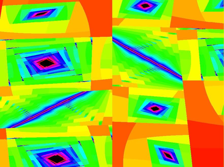
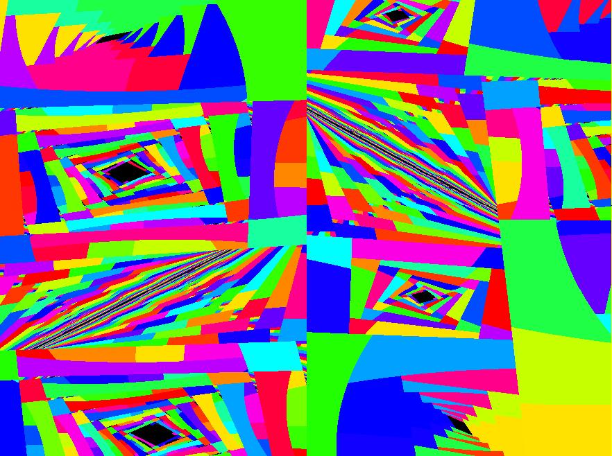
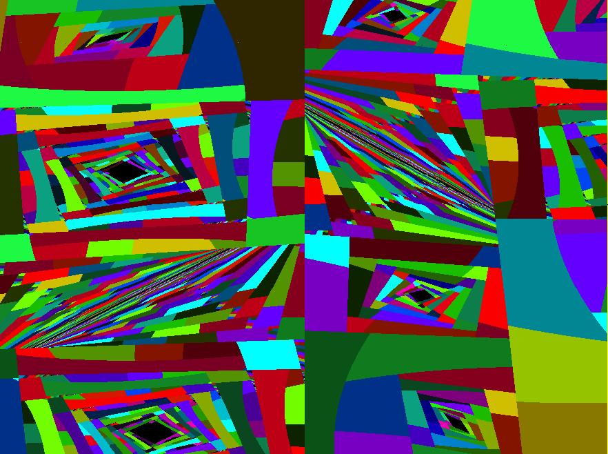
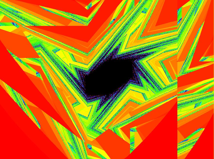
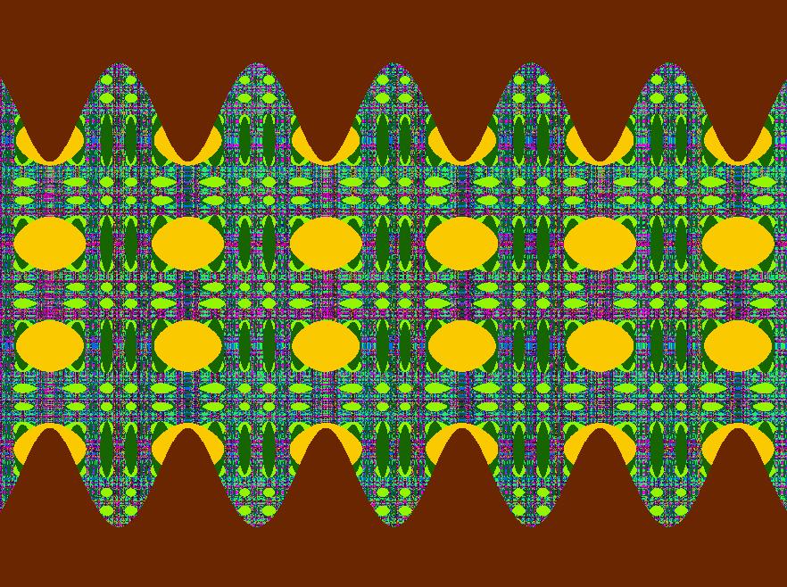
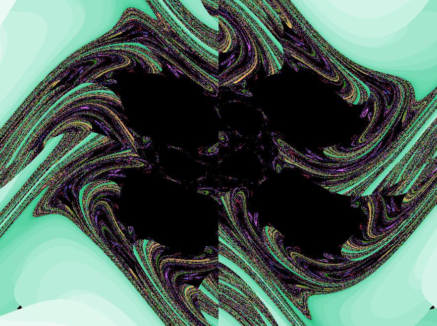
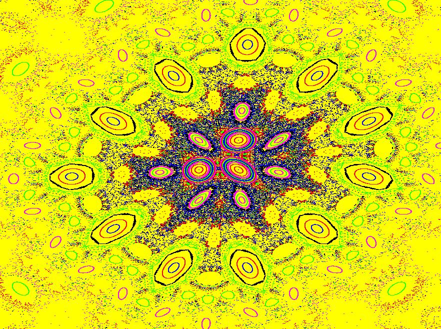
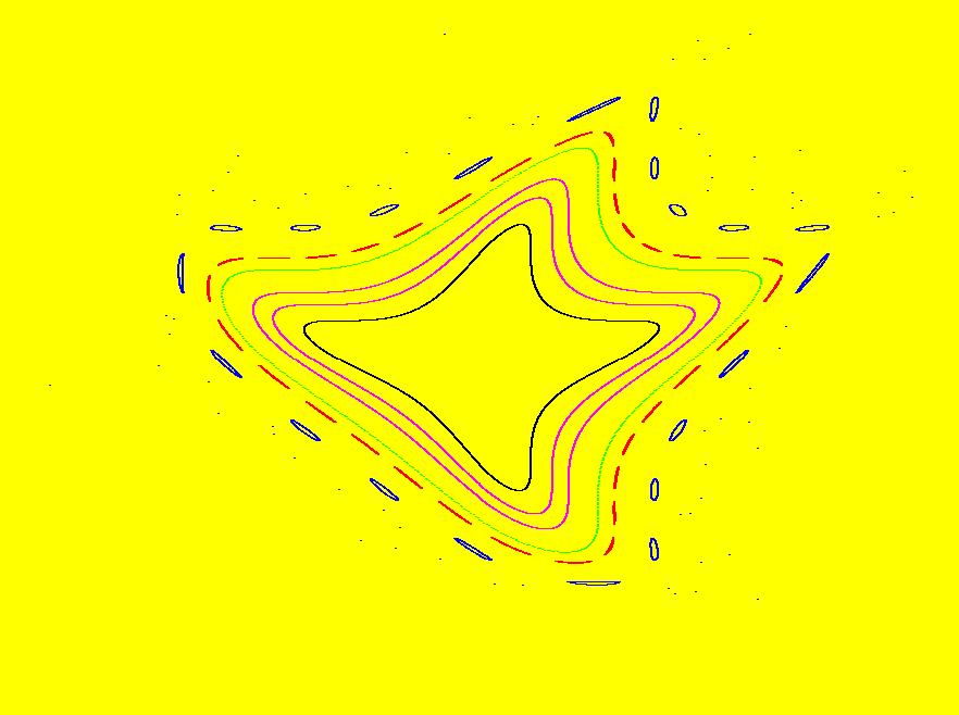
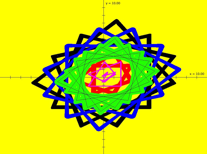
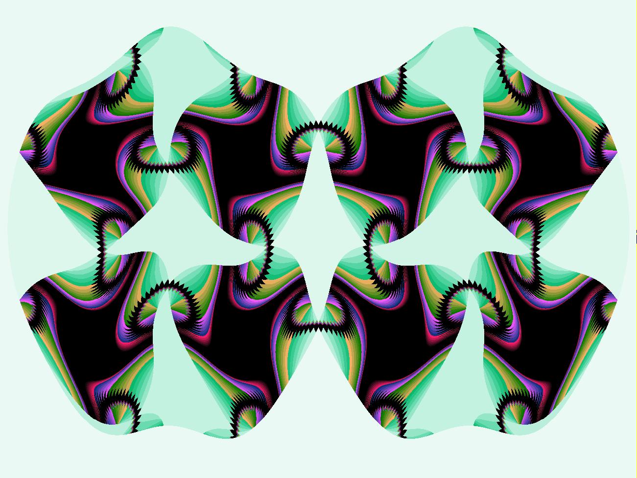
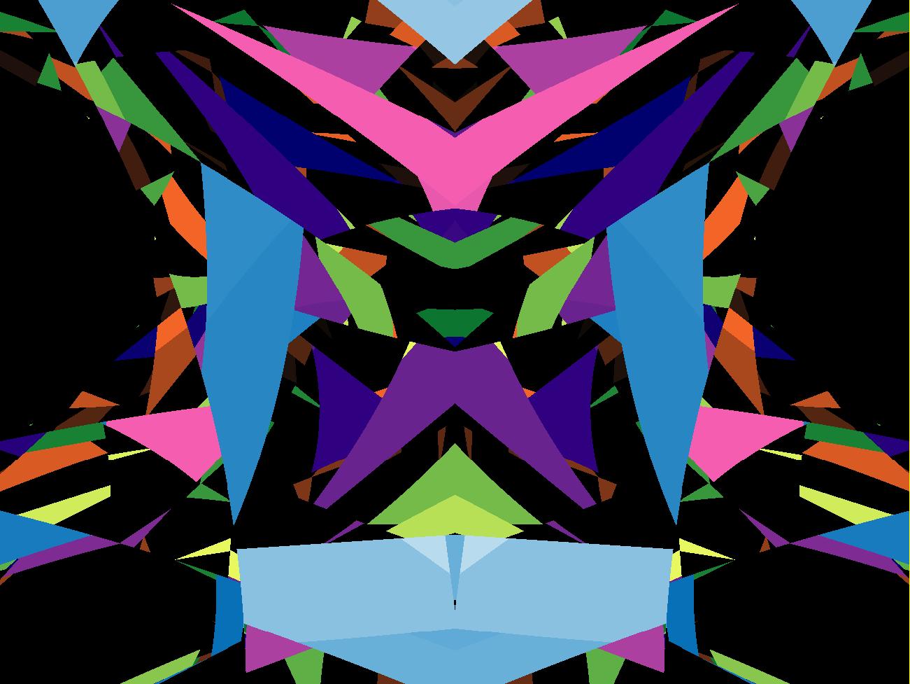
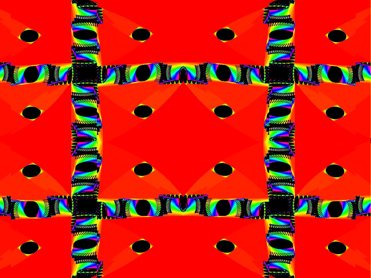
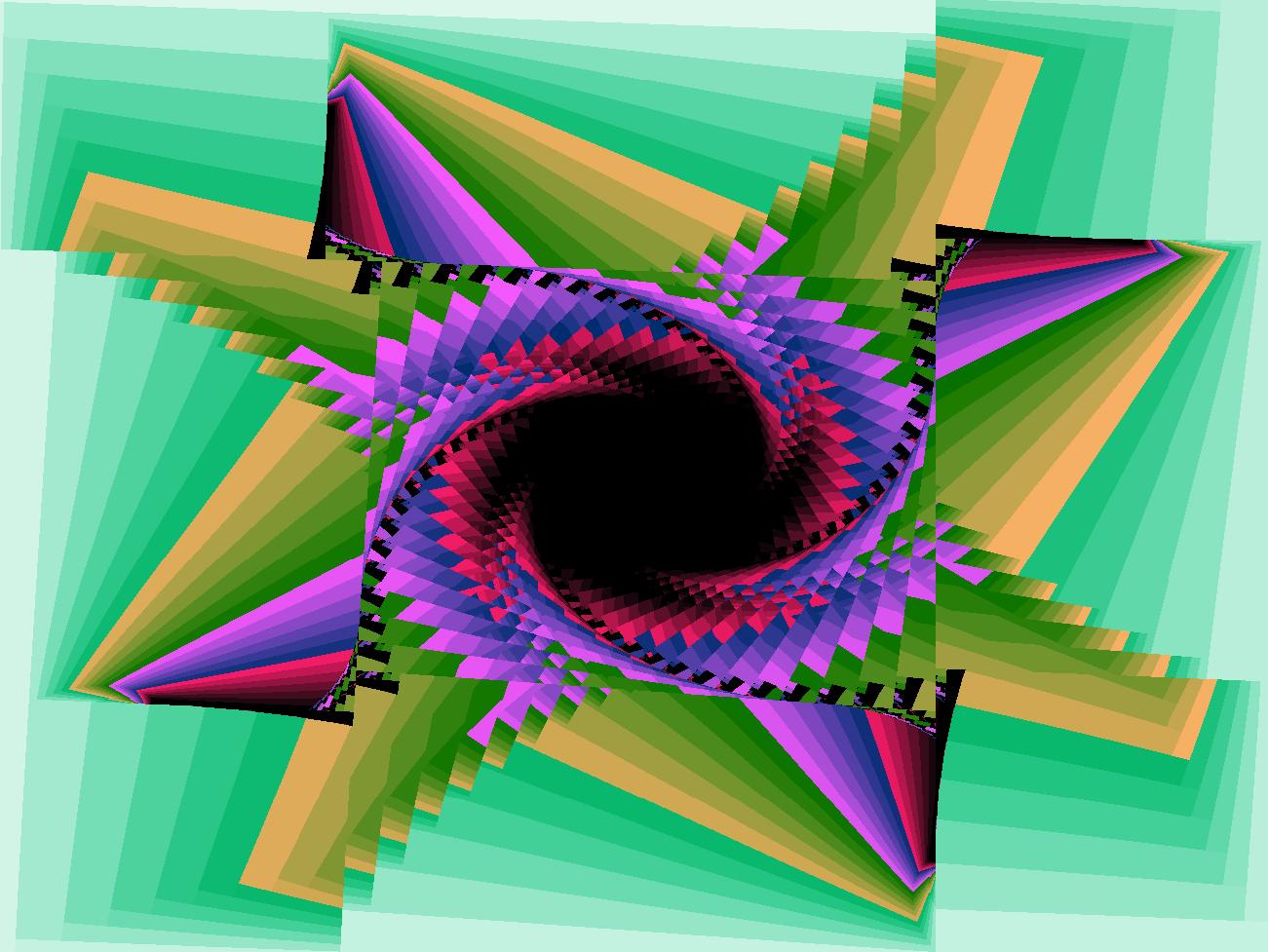
View/Sys/Gal: EMap "2D: ode/IMap0011/emap kaleidoscope" in "MapExs." This iteration is defined by:
x <- y-b*cos(x%d),
y <- a-abs(x%c).
Parameters are:
a = 7.300; b = .030; c = 4.700; d = 2.700;
To generate an interesting family of images, vary the parameters starting with d, then c, then b.
Parameter "a" shifts the image along the lower-left to upper-right diagonal in the viewing area.
Also try the EMap view.
|
|
|
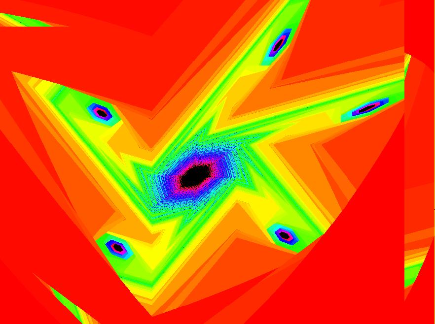
View/Sys/Gal: EMap "2D: ode/IMap0011/emap kaleidoscope w/two orbits" in "MapExs." This iteration is defined by:
x <- y-b*cos(x%d),
y <- a-abs(x%c).
Parameters are:
a = 7.000; b = .044;
c = 4.400; d = -1.300;
This is just two orbits. The blue one starts at
(x,y) = (3.950133,3.980544)
and the red one starts at
(x.y) = (3.660457,2.603861).
Wait for the orbits to appear.
Try adjusting the parameters.
Also see the EMap view. Zoom out a few times.
|
|
|
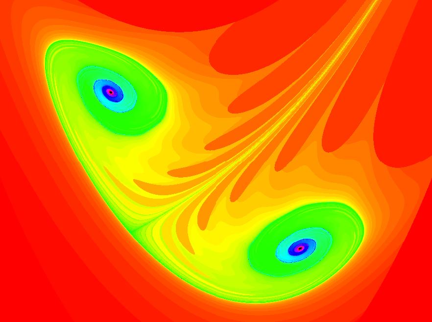
View/Sys/Gal: EMap "2D: ode/imap/EMap ver 3b" in "MapExs." This iteration is defined by:
x <- y-b*cos(x),
y <- a-abs(x).
Parameters are:
a = 6.00; b = .70;
|
|
|
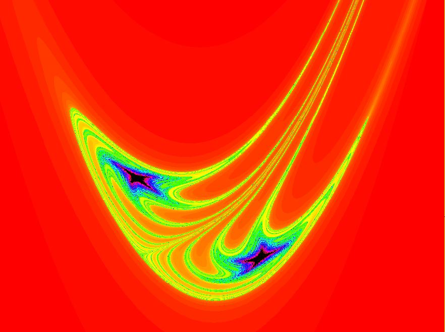
View/Sys/Gal: EMap "2D: ode/imap/EMap ver 4" in "MapExs." This iteration is defined by:
x <- y-b*cos(x),
y <- a-abs(x).
Parameters are:
a = 6.00; b = .78;
|
|
|
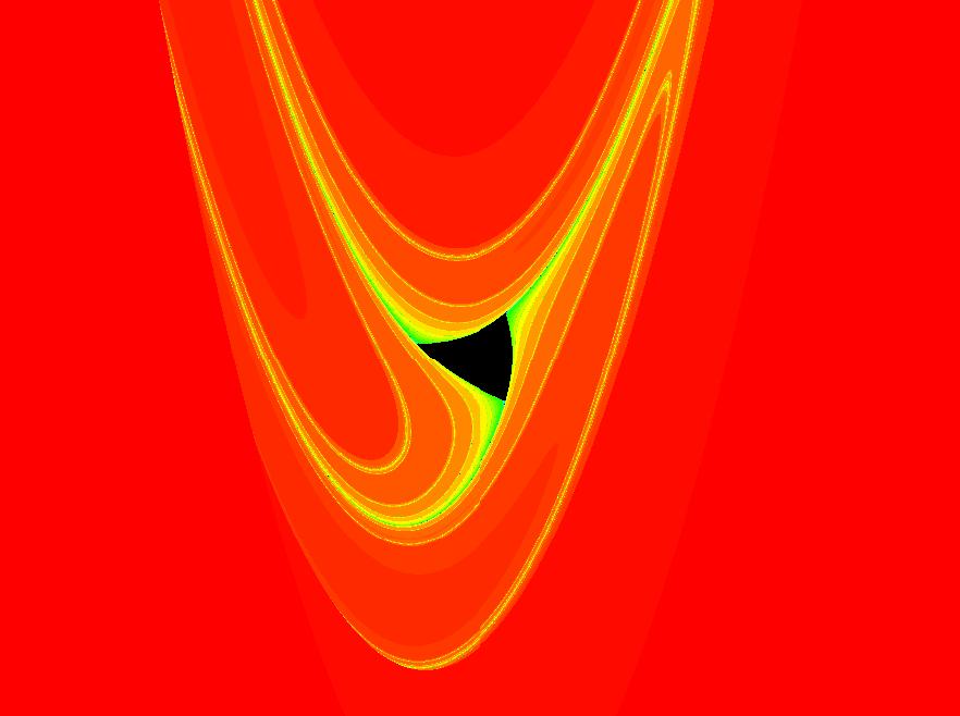
View/Sys/Gal: EMap "2D: ode/imap/EMap ver 5" in "MapExs." This iteration is defined by:
x <- y-b*cos(x),
y <- a-abs(x).
Parameters are:
a = 6.10; b = .47;
|
|
|
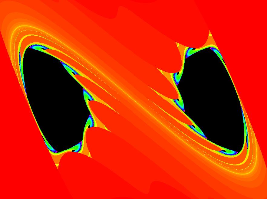
View/Sys/Gal: EMap "2D: ode/imap/EMap ver 5.1" in "MapExs." This iteration is defined by:
x <- y-b*cos(x),
y <- a-abs(x).
Parameters are:
a = 6.10; b = .47;
|
|
|
View/Sys/Gal: EMap "2D: ode/imap/EMap ver 5.2" in "MapExs." This iteration is defined by:
x <- y-b*cos(x),
y <- a-abs(x).
Parameters are:
a = 6.10; b = .47;
|
|
|
View/Sys/Gal: EMap "2D: ode/imap/EMap ver 5.3" in "MapExs." This iteration is defined by:
x <- y-b*cos(x),
y <- a-abs(x).
Parameters are:
a = 6.10; b = .47;
|
|
|
View/Sys/Gal: EMap "2D: ode/imap/EMap ver 5.4" in "MapExs." This iteration is defined by:
x <- y-b*cos(x),
y <- a-abs(x).
Parameters are:
a = 6.10; b = .47;
Right click in the graphics area to see the 4 by 4 quilt image. Click "Center" to return to the original image.
|
|
|
View/Sys/Gal: EMap "2D: ode/imap/EMap ver 5.5" in "MapExs." This iteration is defined by:
x <- y-b*cos(x),
y <- a-abs(x).
Parameters are:
a = -.100; b = .150;
|
|
|
View/Sys/Gal: EMap "2D: ode/imap/EMap ver 6" in "MapExs." This iteration is defined by:
x <- y-b*cos(x),
y <- a-abs(x%c).
Parameters are:
a = 6.10; b = .54; c = 5.40;
|
|
|
View/Sys/Gal: EMap "2D: ode/imap/EMap ver 6.1" in "MapExs." This iteration is defined by:
x <- y-b*cos(x),
y <- a-abs(x%c).
Parameters are:
a = 6.10; b = .54; c = 5.40;
|
|
|
View/Sys/Gal: EMap "2D: ode/imap/EMap ver 6.2" in "MapExs." This iteration is defined by:
x <- y-b*cos(x),
y <- a-abs(x%c).
Parameters are:
a = 6.10; b = .54; c = 5.40;
|
|
|
View/Sys/Gal: EMap "2D: ode/imap/EMap ver 7" in "MapExs." This iteration is defined by:
x <- y-b*cos(x%d),
y <- a-abs(x%c).
Parameters are:
a = 6.10; b = .53; c = 4.70; d = 2.70;
|
|
|
View/Sys/Gal: EMap "2D: ode/imap/EMap ver 7.1" in "MapExs." This iteration is defined by:
x <- (1+.001*s)*(y-b*cos(x%d)),
y <- (1+.001*s)*(a-abs(x%c)).
Parameters are:
a = 6.10; b = .55; c = 7.50;
d = 4.00; s = 38.00;
|
|
|
View/Sys/Gal: EMap "2D: ode/imap/EMap ver 7.2" in "MapExs." This iteration is defined by:
x <- (1+.001*s)*(y-b*cos(x%d)),
y <- (1+.001*s)*(a-abs(x%c)).
Parameters are:
a = 6.10; b = .53; c = 4.70;
d = 2.70; s=0
|
|
|
View/Sys/Gal: EMap "2D: ode/imap/EMap ver 7.3" in "MapExs." This iteration is defined by:
x <- y-b*cos(x%d),
y <- a-abs(x%c).
Parameters are:
a = 6.10; b = .53; c = 4.70; d = 2.70;
|
|
|
View/Sys/Gal: EMap "2D: ode/imap/EMap ver 7.5" in "MapExs." This iteration is defined by:
x <- y-b*cos(x%d),
y <- a-abs(x%c).
Parameters are:
a = 7.300; b = .031; c = 4.800; d = 2.700;
|
|
|
View/Sys/Gal: EMap "2D: ode/imap/EMap ver 7.6" in "MapExs." This iteration is defined by:
x <- y-b*cos(x%d),
y <- a-abs(x%c).
Parameters are:
a = 6.100; b = .085; c = 3.500; d = 2.700;
|
|
|
View/Sys/Gal: EMap "2D: ode/imap/EMap ver 7.6b" in "MapExs." This iteration is defined by:
x <- y-b*cos(x%d),
y <- a-abs(x%c).
Parameters are:
a = 6.100; b = .085; c = 3.500; d = 2.700;
|
|
|
View/Sys/Gal: EMap "2D: ode/imap/EMap ver 7.6c" in "MapExs." This iteration is defined by:
x <- y-b*cos(x%d),
y <- a-abs(x%c).
Parameters are:
a = 6.100; b = .085; c = 3.500; d = 2.700;
|
|
|
View/Sys/Gal: EMap "2D: ode/imap/EMap ver 7.6d" in "MapExs." This iteration is defined by:
x <- y-b*cos(x%d),
y <- a-abs(x%c).
Parameters are:
a = 6.000; b = .087; c = 3.300; d = 2.700;
|
|
|
View/Sys/Gal: EMap "2D: ode/imap/EMap ver 7.7" in "MapExs." This iteration is defined by:
x <- y-b*cos(x%d),
y <- a-abs(x%c).
Parameters are:
a = 6.100; b = .085; c = 3.500; d = 2.700;
|
|
|
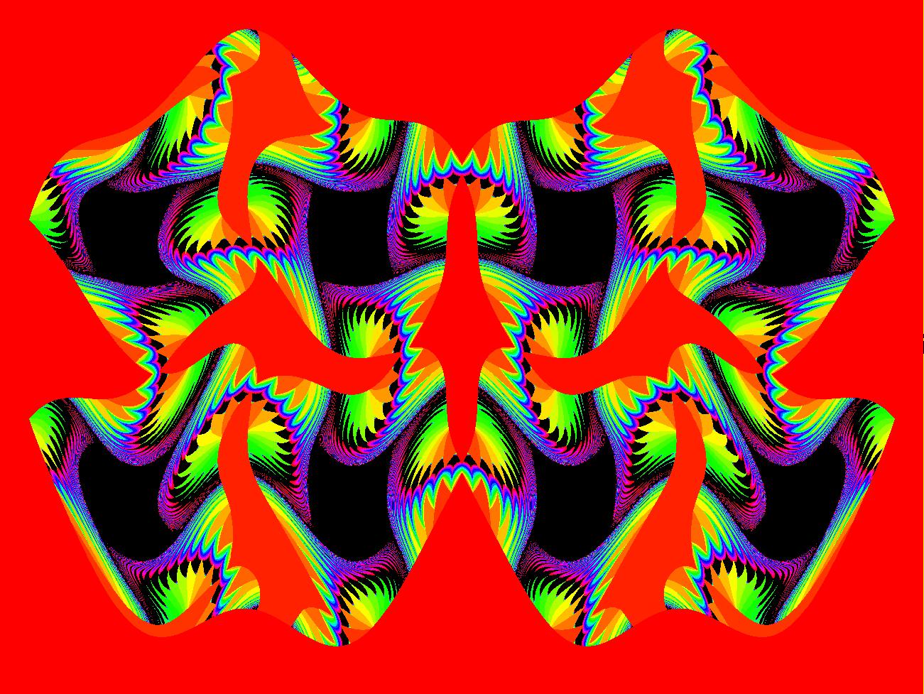
View/Sys/Gal: EMap "2D: ode/imap/EMapCT2 ver 8" in "MapExs." This iteration is defined by:
x <- (1+.1*s)*(y-b*cos(x%d)),
y <- (1+.1*s)*(a-abs(x%c)).
Parameters are:
a = 7.300; b = .058; c = 4.700; d = -1.400; s = .150;
EMap CT: 2
|
|
|
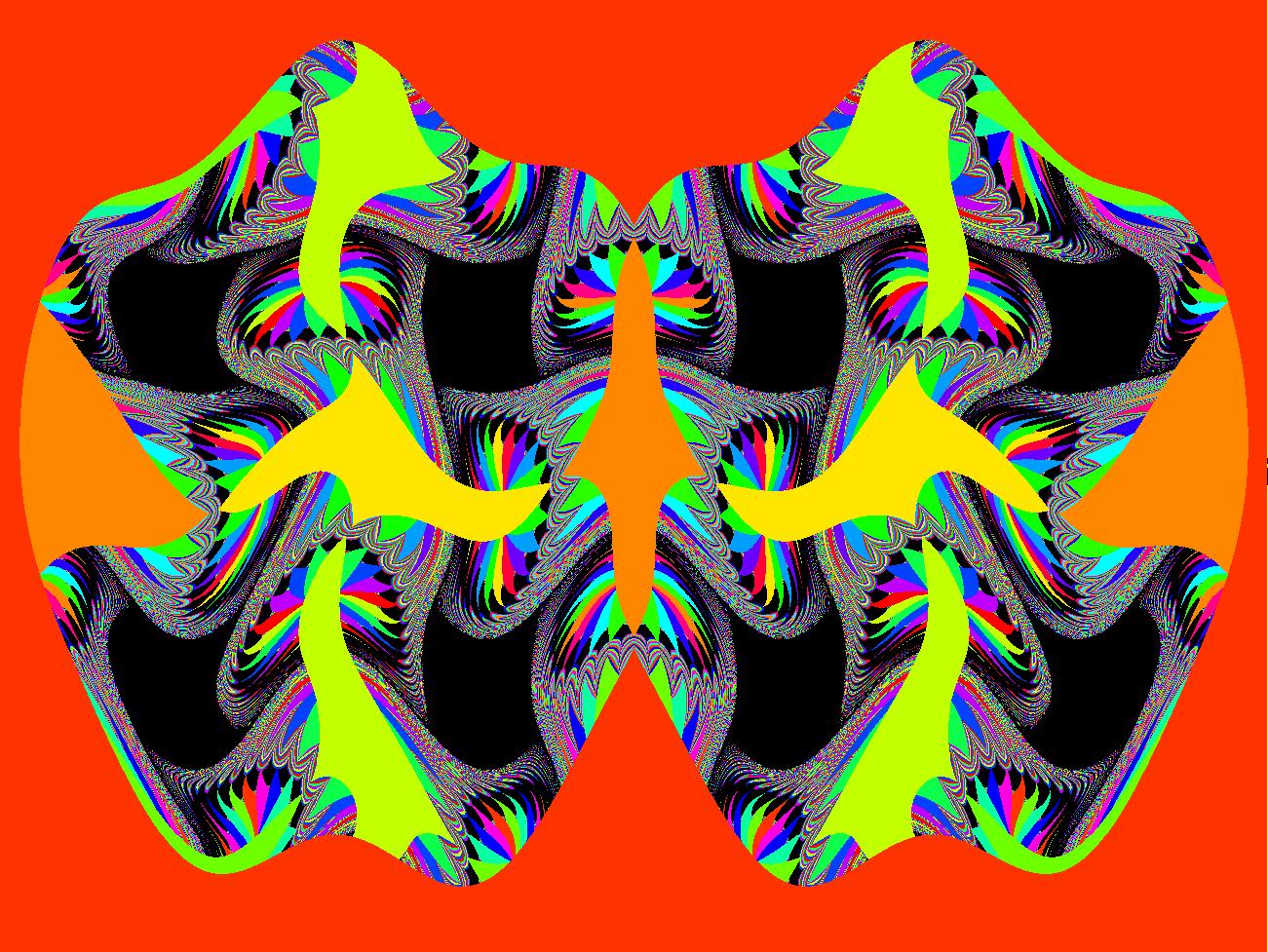
View/Sys/Gal: EMap "2D: ode/imap/EMapCT3 ver 8.1" in "MapExs." This iteration is defined by:
x <- y-b*cos(x%d),
y <- a-abs(x%c).
Parameters are:
a = 7.200; b = .046; c = 4.000; d = -1.400;
EMap CT: 3
|
|
|
View/Sys/Gal: EMap "2D: ode/imap/EMapCT3 ver 8.2" in "MapExs." This iteration is defined by:
x <- y-b*cos(x%d),
y <- a-abs(x%c).
Parameters are:
a = 7.200; b = .048; c = 4.100; d = -1.400;
EMap CT: 3
|
|
|
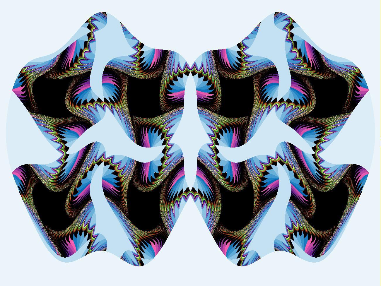
View/Sys/Gal: EMap "2D: ode/imap/EMapCT6 ver 8.3" in "MapExs." This iteration is defined by:
x <- (1+.1*s)*(y-b*cos(x%d)),
y <- (1+.1*s)*(a-abs(x%c)).
Parameters are:
a = 7.300; b = .048; c = 4.400; d = -2.000; s = .150;
EMap CT: 6
|
|
|
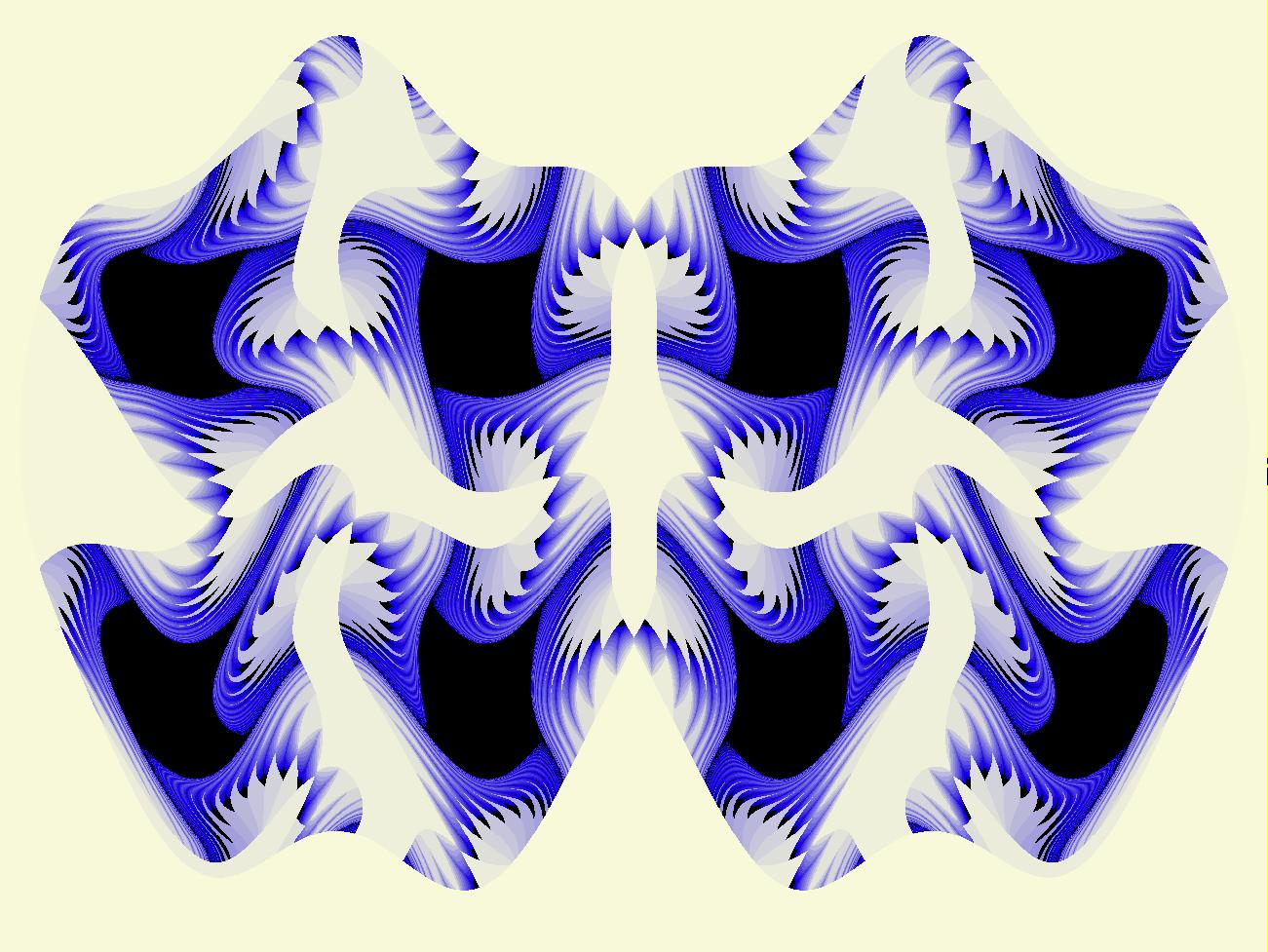
View/Sys/Gal: EMap "2D: ode/imap/EMapCT7 ver 8.4" in "MapExs." This iteration is defined by:
x <- (1+.1*s)*(y-b*cos(x%d)),
y <- (1+.1*s)*(a-abs(x%c)).
Parameters are:
a = 7.200; b = .048; c = 4.400; d = -2.000; s = .150;
EMap CT: 7
|
|
|
View/Sys/Gal: EMap "2D: ode/imap/EMapCT7 ver 8.5" in "MapExs." This iteration is defined by:
x <- (1+.1*s)*(y-b*cos(x%d)),
y <- (1+.1*s)*(a-abs(x%c)).
Parameters are:
a = 7.200; b = .048; c = 4.400; d = -2.000; s = .150;
EMap CT: 7
|
|
|
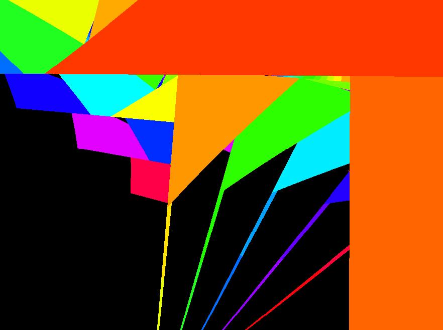
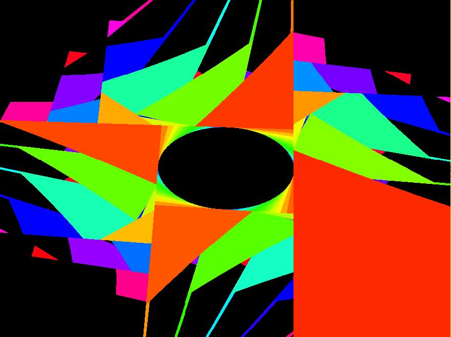
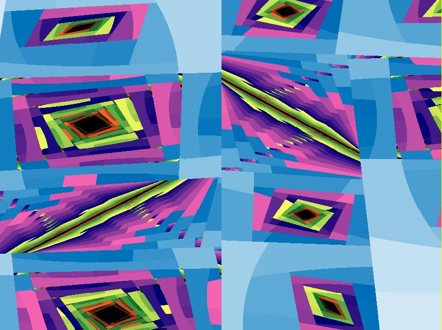
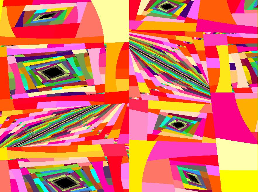
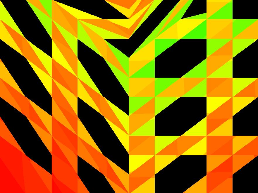
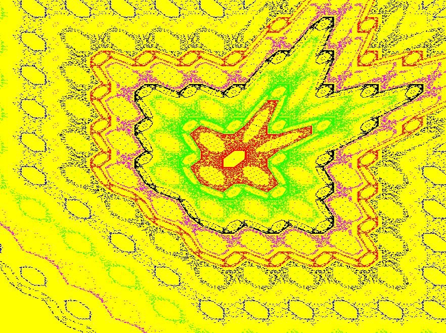
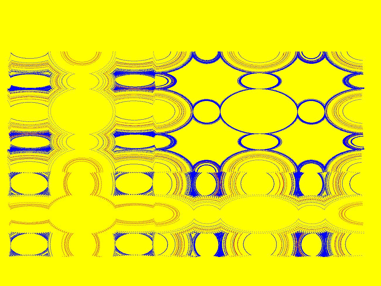
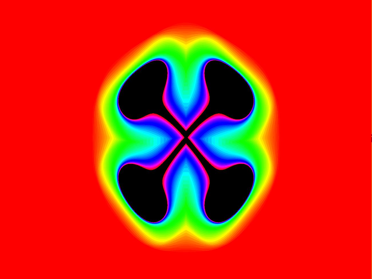
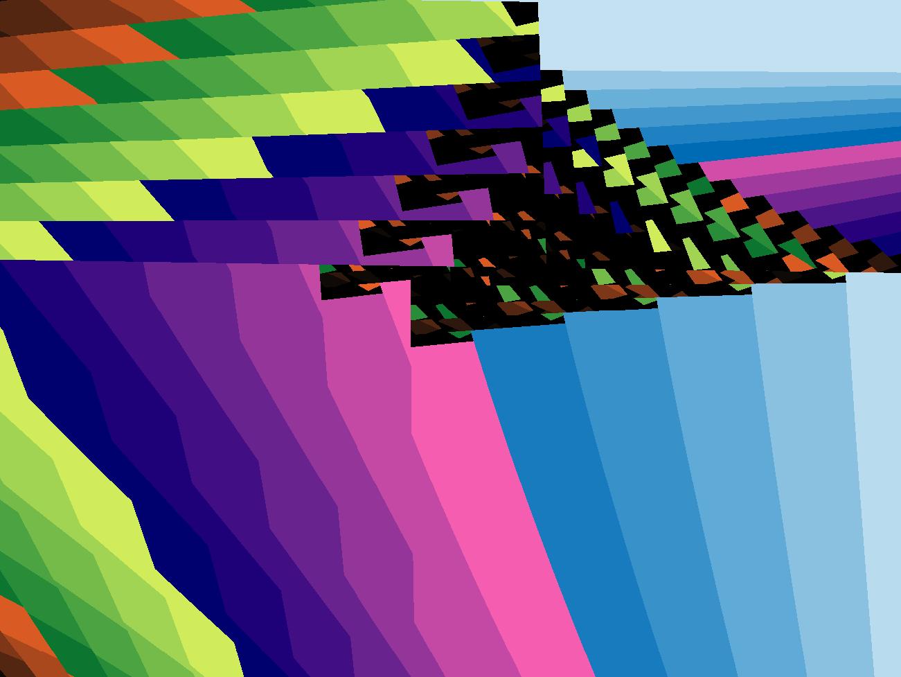
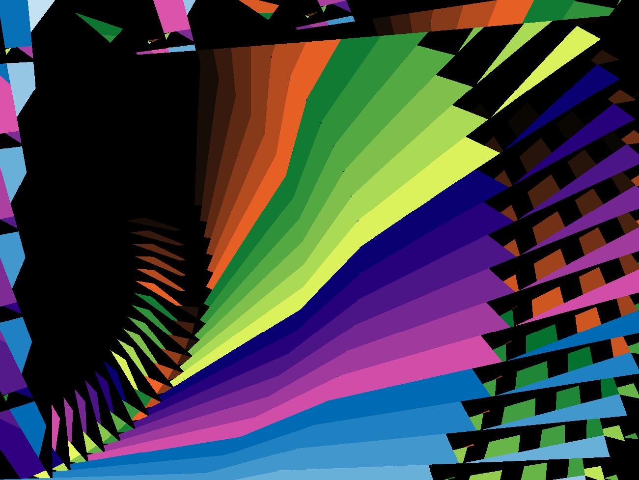
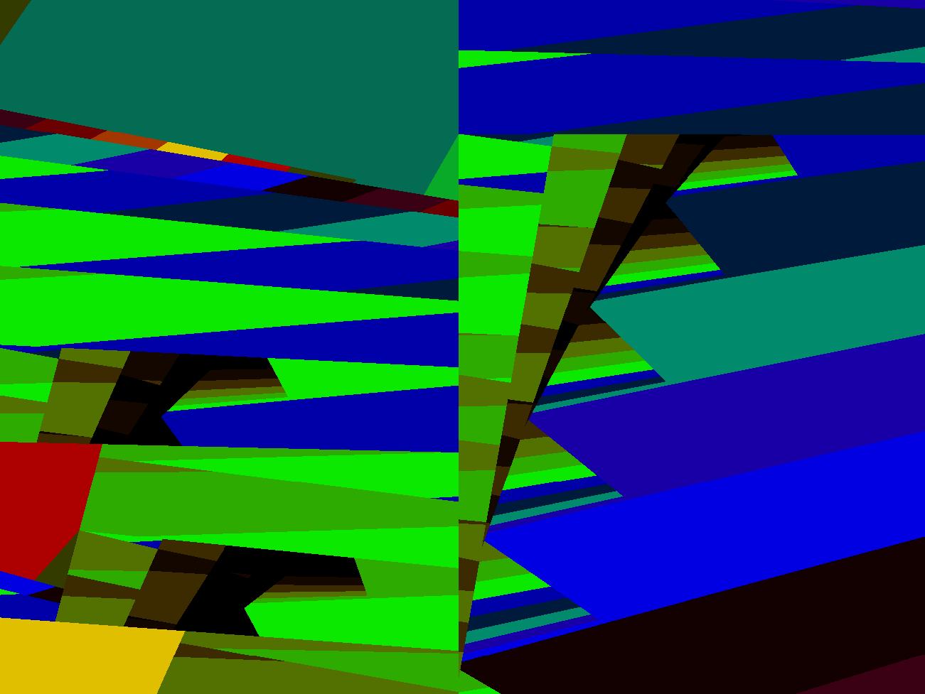
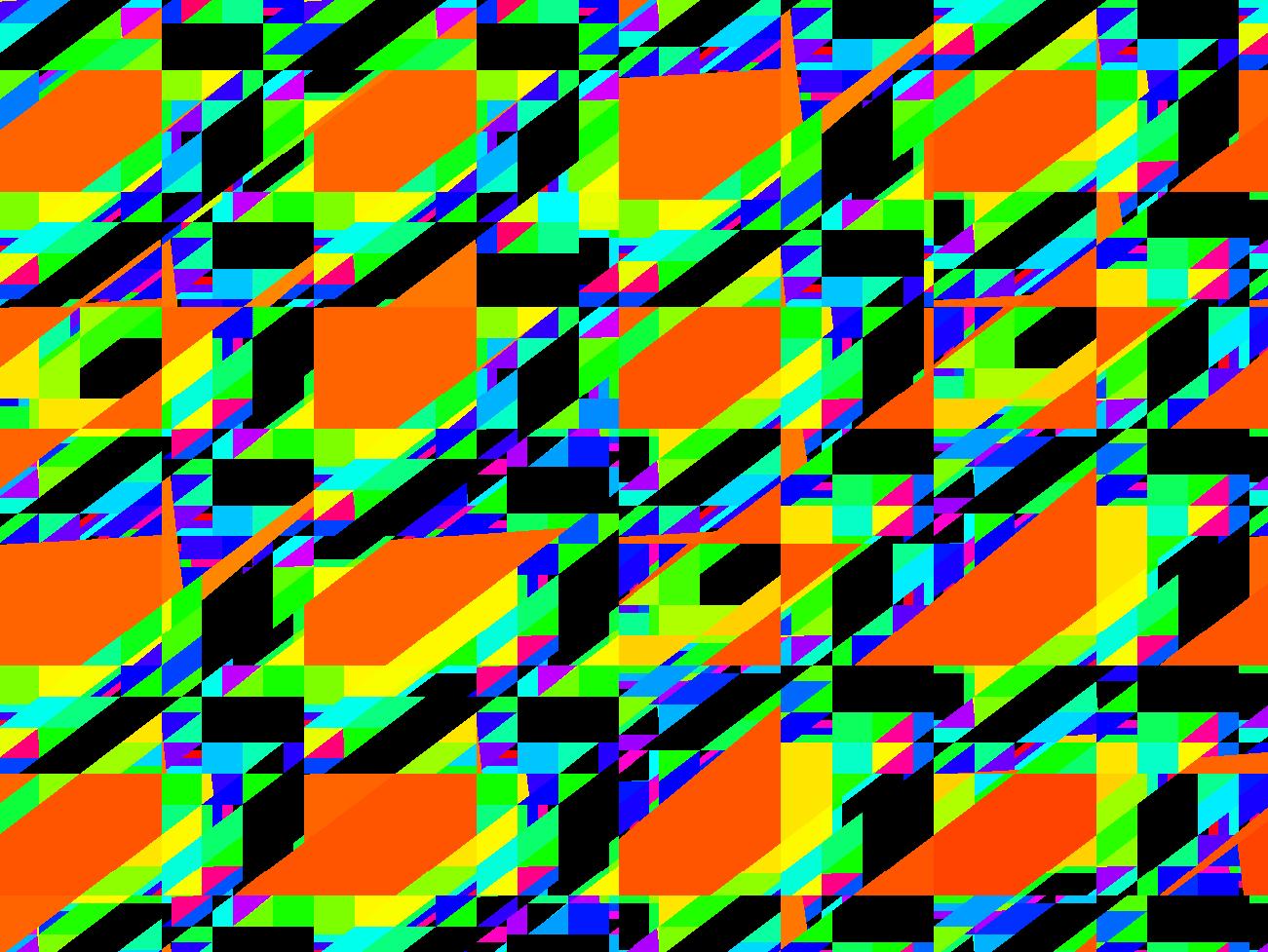
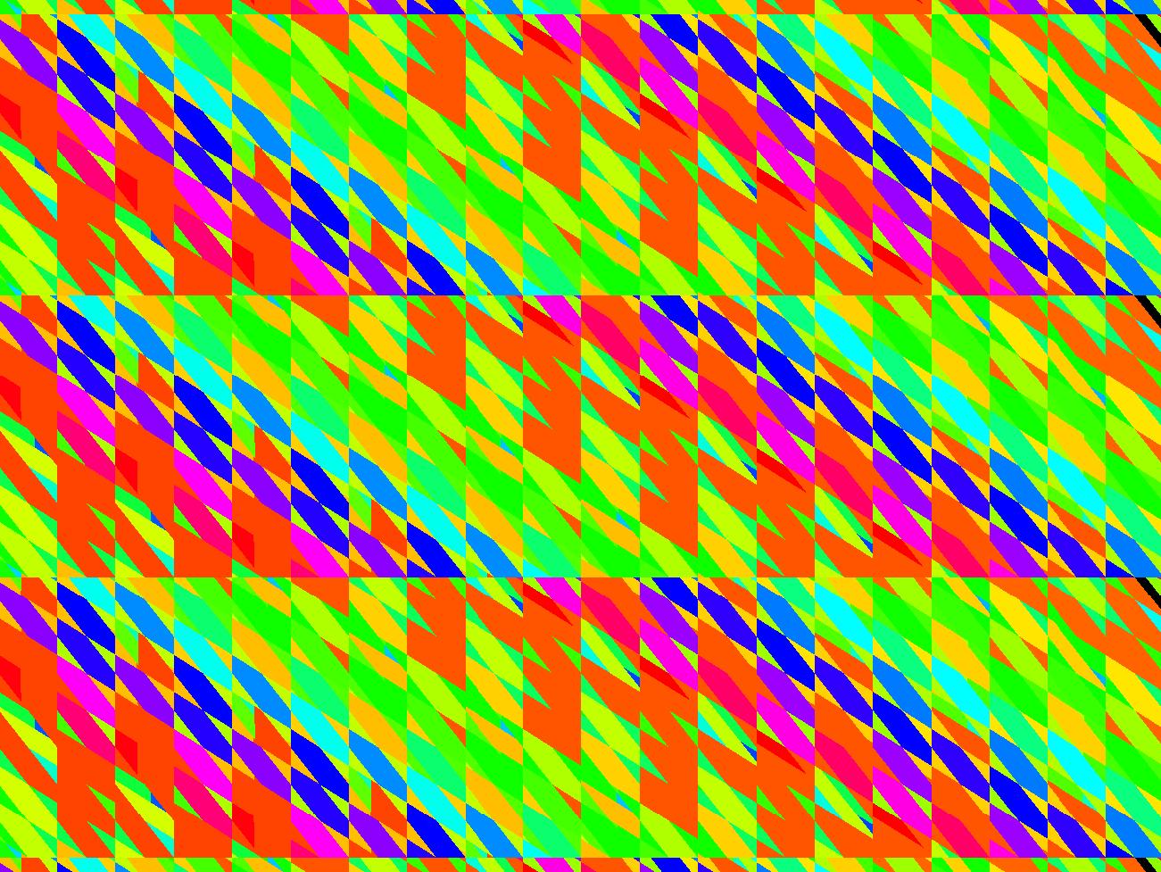
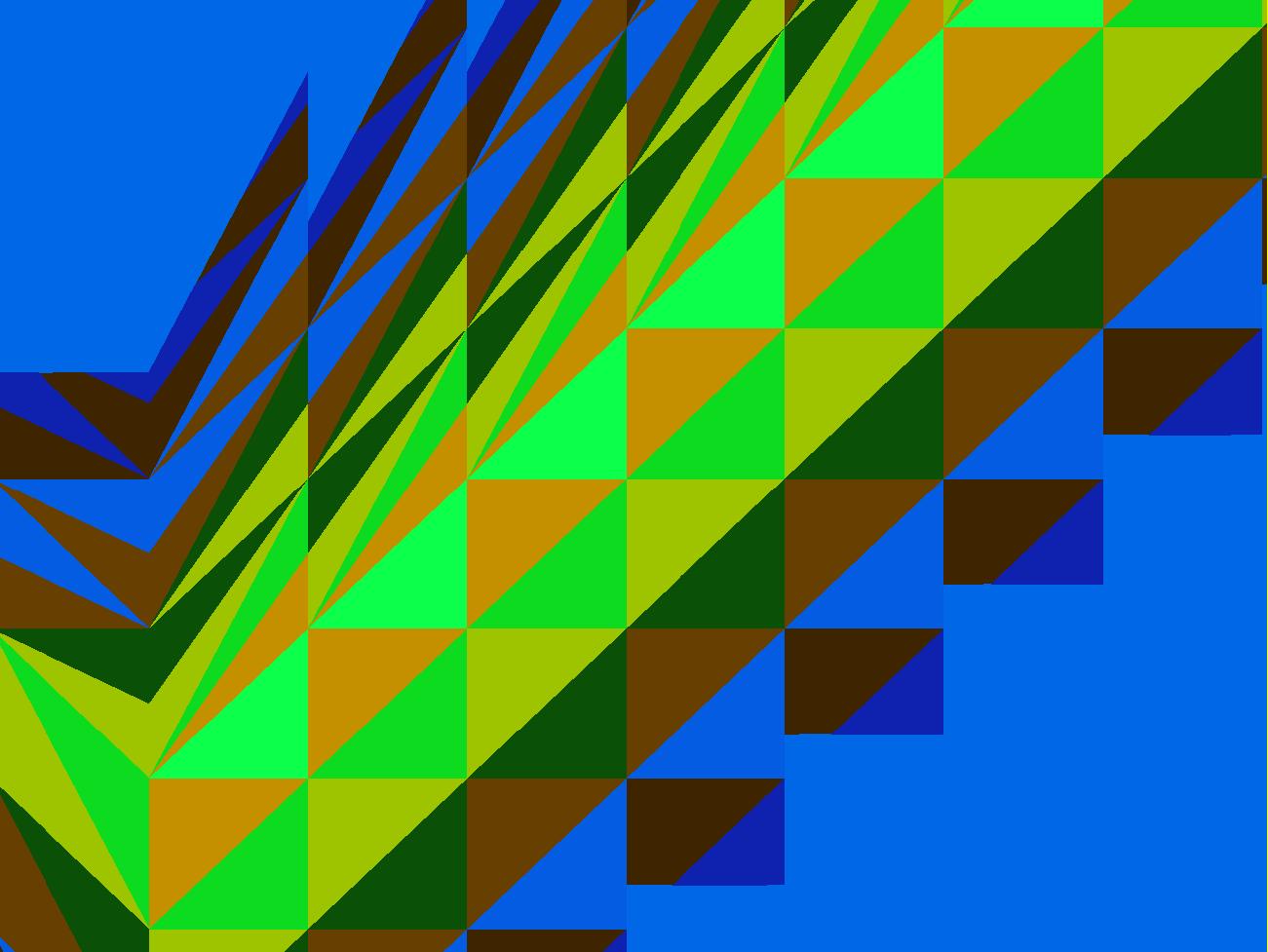
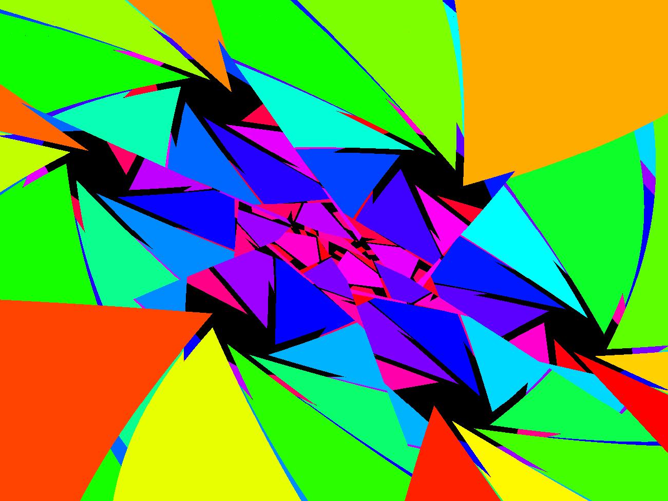
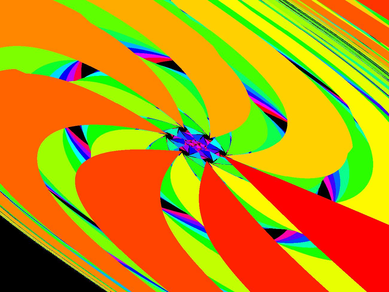
View/Sys/Gal: EMap "Geometric Image: ( 1) EMap" in "MapExs." This system of odes is defined by the equations:
dx/dt = 1-y%b+abs(x%a),
dy/dt = x%c
Parameters are:
a = 6.70; b = .60; c = .92;
Zoom out to see the rest of the EMap.
This is the starting image in a series of images. The images are variations arrived at by modifying the parameters, zooming in/out and selecting parts of this first images.
The introduction of the Java mod operator, %, and the absolute value function, in the underlying linear system produces four non-commensurate periodicities in the dynamics of this otherwise linear system.
|
|
|
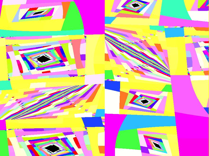
View/Sys/Gal: EMap "Geometric Image: ( 2) EMapCT3" in "MapExs." This iteration is defined by:
x <- 1-y%b+abs(x%a),
y <- x%c.
Parameters are:
a = 6.400; b = .600; c = .920;
EMap CT: 3
Parameter "a" was just decreased a bit to generate this image.
|
|
|
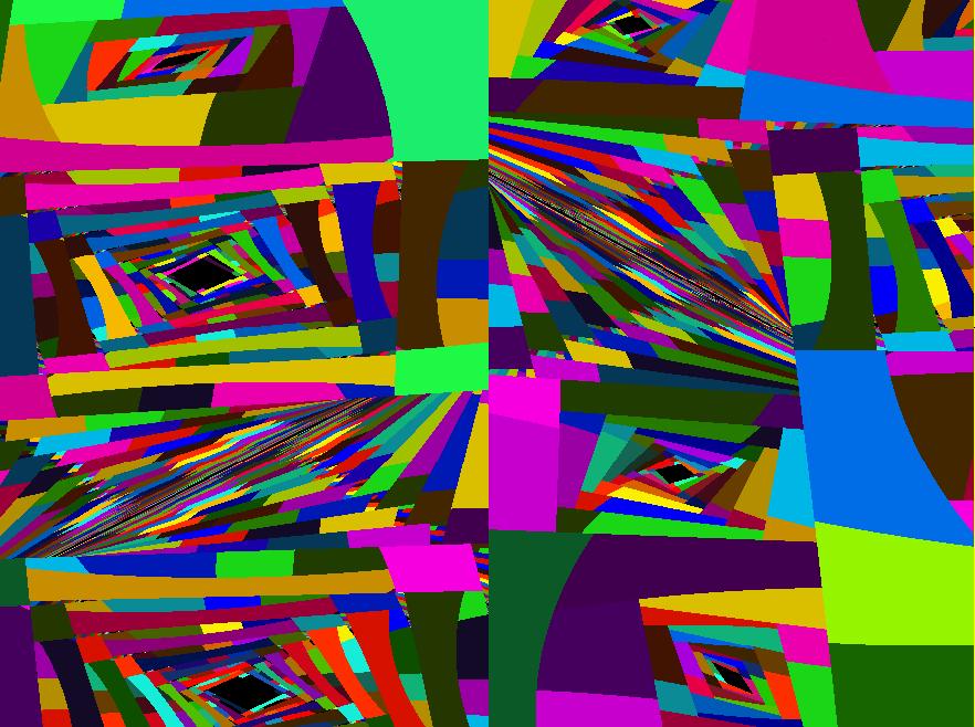
View/Sys/Gal: EMap "Geometric Image: ( 3) EMap" in "MapExs." This iteration is defined by:
x <- 1-y%b+abs(x%a),
y <- x%c.
Parameters are:
a = 6.400; b = .610; c = .920;
EMap CT: 0
Here, b was increased a bit.
|
|
|
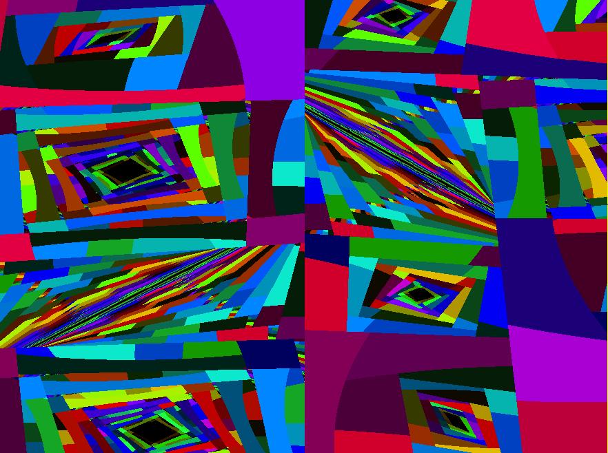
View/Sys/Gal: EMap "Geometric Image: ( 4) EMapCT5" in "MapExs." This iteration is defined by:
x <- 1-y%b+abs(x%a),
y <- x%c.
Parameters are:
a = 6.400; b = .610; c = -.200;
EMap CT: 5
Parameter c was changed to -.2 to get to this image.
|
|
|
View/Sys/Gal: EMap "Geometric Image: ( 5) EMap" in "MapExs." This iteration is defined by:
x <- 1-y%b+abs(x%a),
y <- x%c.
Parameters are:
a = 6.400; b = .610; c = -.420;
EMap CT: 0
Here c is -.42.
|
|
|
View/Sys/Gal: EMap "Geometric Image: ( 6) EMap" in "MapExs." This iteration is defined by:
x <- 1-y%b+abs(x%a),
y <- x%c.
Parameters are:
a = 6.400; b = .610; c = -.570;
EMap CT: 0
Here c is -.57.
|
|
|
View/Sys/Gal: EMap "Geometric Image: ( 7) EMap" in "MapExs." This iteration is defined by:
x <- 1-y%b+abs(x%a),
y <- x%c.
Parameters are:
a = 6.400; b = .610; c = -.570;
EMap CT: 0
The previous image was zoomed out then a part of the image to the left was selected and enlarged.
|
|
|
View/Sys/Gal: EMap "Geometric Image: ( 8) EMapCT7" in "MapExs." This iteration is defined by:
x <- 1-y%b+abs(x%a),
y <- x%c.
Parameters are:
a = 6.400; b = .610; c = -.570;
EMap CT: 7
This is part of the previous image after a selection and zoom in.
|
|
|
View/Sys/Gal: EMap "Geometric Image: ( 9) EMap" in "MapExs." This iteration is defined by:
x <- 1-y%b+abs(x%a),
y <- x%c.
Parameters are:
a = 6.400; b = .610; c = -.160;
EMap CT: 0
Parameter c was changed.
|
|
|
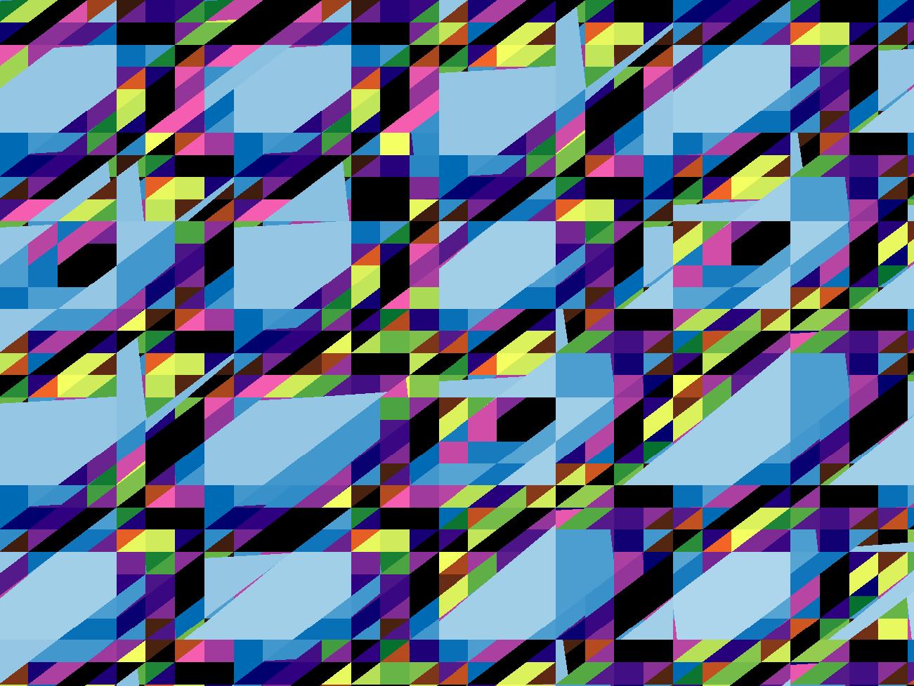
View/Sys/Gal: EMap "Geometric Image: (10) EMapCT2" in "MapExs." This iteration is defined by:
x <- 1-y%b+abs(x%a),
y <- x%c.
Parameters are:
a = 6.200; b = 5.700; c = -.080;
EMap CT: 2
Parameters a, b and c were changed.
|
|
|
View/Sys/Gal: EMap "Geometric Image: (11) EMapCT3" in "MapExs." This iteration is defined by:
x <- 1-y%b+abs(x%a),
y <- x%c.
Parameters are:
a = 6.400; b = 5.700; c = -.080;
EMap CT: 3
Parameter a was changed.
|
|
|
View/Sys/Gal: EMap "Geometric Image: (12) EMap" in "MapExs." This iteration is defined by:
x <- 1-y%b+abs(x%a),
y <- x%c.
Parameters are:
a = 6.400; b = 5.700; c = -.080;
EMap CT: 0
Image was zoomed out and centered.
|
|
|
View/Sys/Gal: EMap "Geometric Image: (13) EMapCT2" in "MapExs." This iteration is defined by:
x <- 1-y%b+abs(x%a),
y <- x%c.
Parameters are:
a = 6.700; b = 5.700; c = -.100;
EMap CT: 2
Parameters were changed a bit, image was zoomed, vMax and vMin were changed.
|
|
|
View/Sys/Gal: EMap "Geometric Image: (14) EMapCT5" in "MapExs." This iteration is defined by:
x <- 1-y%b+abs(x%a),
y <- x%c.
Parameters are:
a = 6.700; b = 5.700; c = -.100;
EMap CT: 5
Part of previous image.
Right click in graphics area for a shifted quilt pattern.
|
|
|
View/Sys/Gal: EMap "Geometric Image: (15) EMapCT6" in "MapExs." This iteration is defined by:
x <- 1-y%b+abs(x%a),
y <- x%c.
Parameters are:
a = 6.500; b = .400; c = .470;
EMap CT: 6
Yet another "random" image.
|
|
|
View/Sys/Gal: EMap "Geometric Image: (16) EMap" in "MapExs." This iteration is defined by:
x <- 1-y%b+abs(x%a),
y <- x%c.
Parameters are:
a = 6.600; b = .400; c = .470;
EMap CT: 0
Shifted, cropped and "a" adjusted.
|
|
|
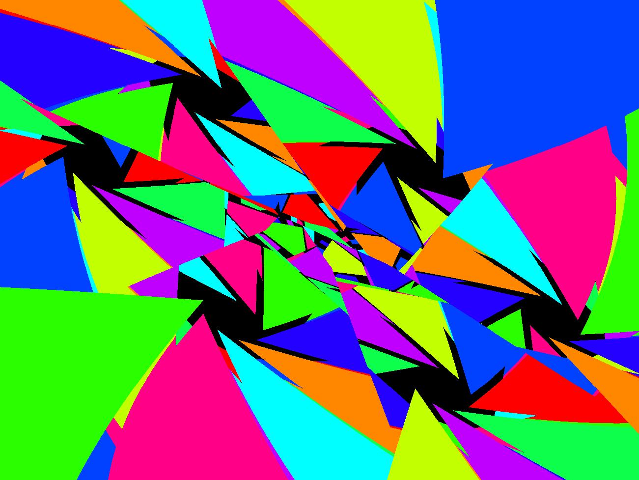
View/Sys/Gal: EMap "Geometric Image: (17) EMapCT5" in "MapExs." This iteration is defined by:
x <- 1-y%b+abs(x%a),
y <- x%c.
Parameters are:
a = 6.600; b = .400; c = .480;
EMap CT: 5
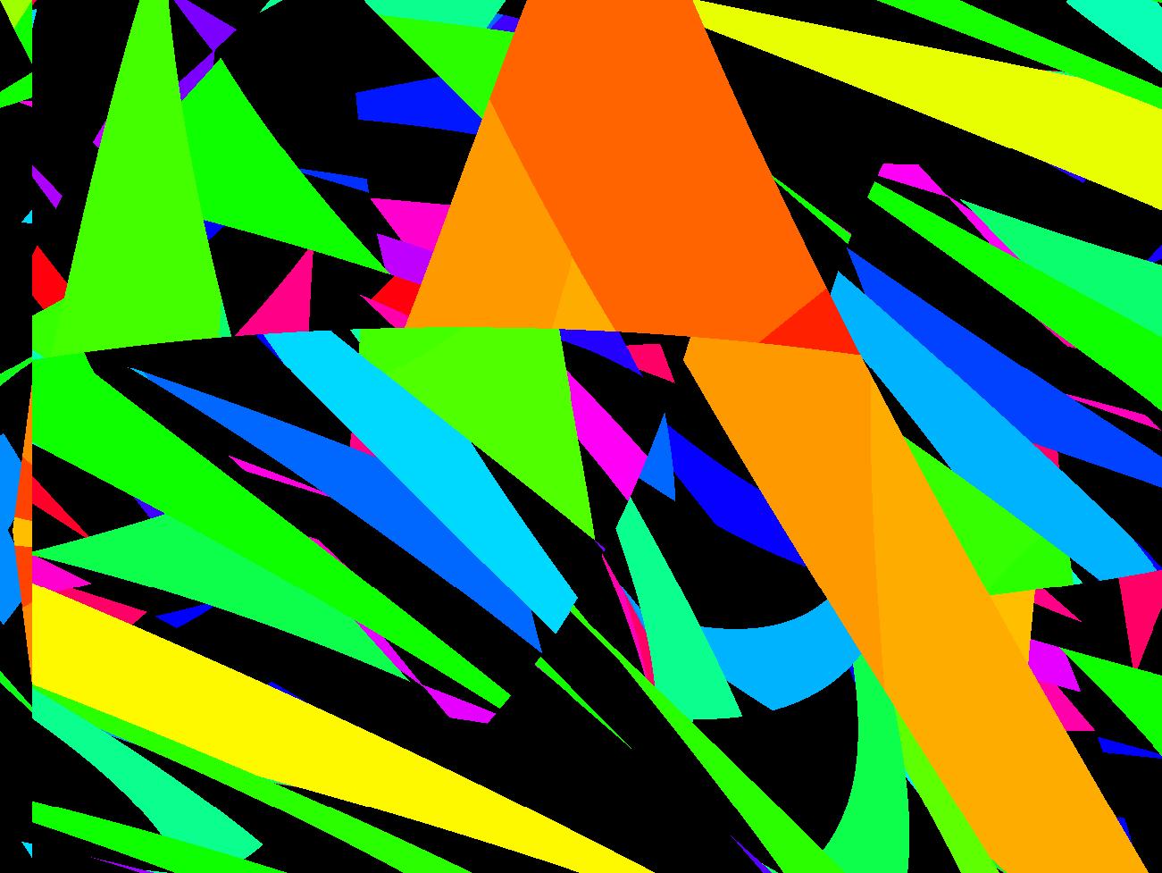
Triangles, squares and parallepipeds.
|
|
|
View/Sys/Gal: EMap "Geometric Image: (18) EMap" in "MapExs." This iteration is defined by:
x <- 1-y%b+abs(x%a),
y <- x%c.
Parameters are:
a = 6.600; b = .400; c = -.410;
EMap CT: 0
More geometric figures.
|
|
|
View/Sys/Gal: EMap "Geometric Image: (19) EMap" in "MapExs." This iteration is defined by:
x <- 1-y%b+abs(x%a),
y <- x%c.
Parameters are:
a = 6.700; b = .600; c = .920;
EMap CT: 0
|
|
|
View/Sys/Gal: IMap "StandardMap: ( 1) IMap0011 (x+k*sin(y),x+y+k*sin(y)), k=1" in "MapExs." This iteration is defined by:
x <- x+k*sin(y),
y <- x+y+k*sin(y).
Parameters are:
k=1
|
|
|
View/Sys/Gal: IMap "StandardMap: ( 2) IMap1000 (x+k*sin(y),x+y+k*sin(y)), k = 2.100; " in "MapExs." This iteration is defined by:
x <- x+k*sin(y),
y <- x+y+k*sin(y).
Parameters are:
k = 2.100;
A period-1 orbit (fixed point) at
(0.000000,3.141667) and
a period-4 orbit at
(1.076736,-2.603258).
|
|
|
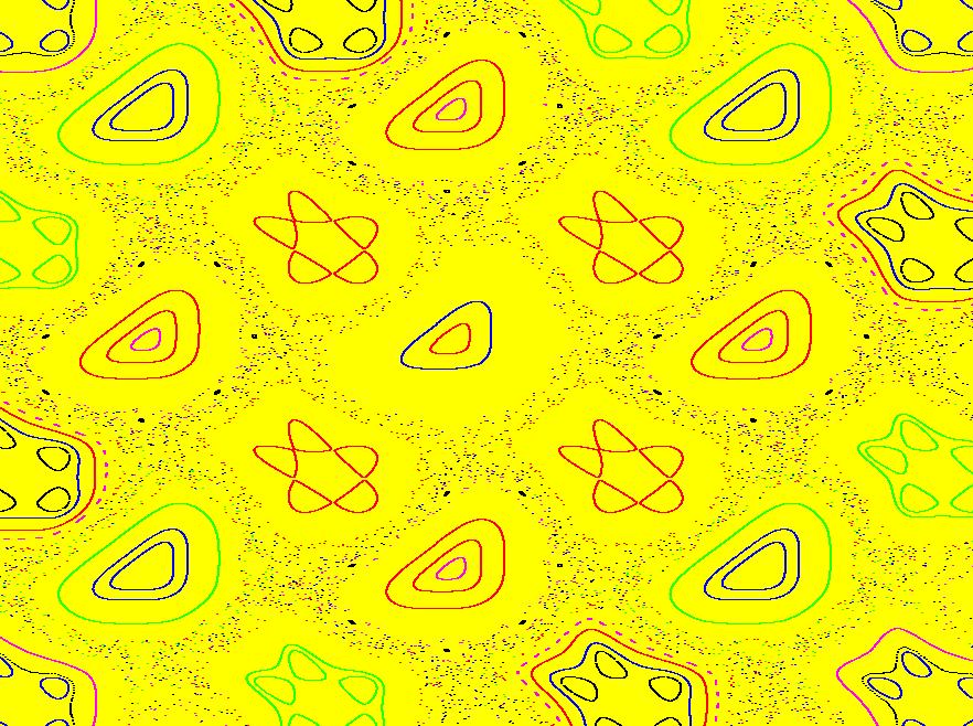
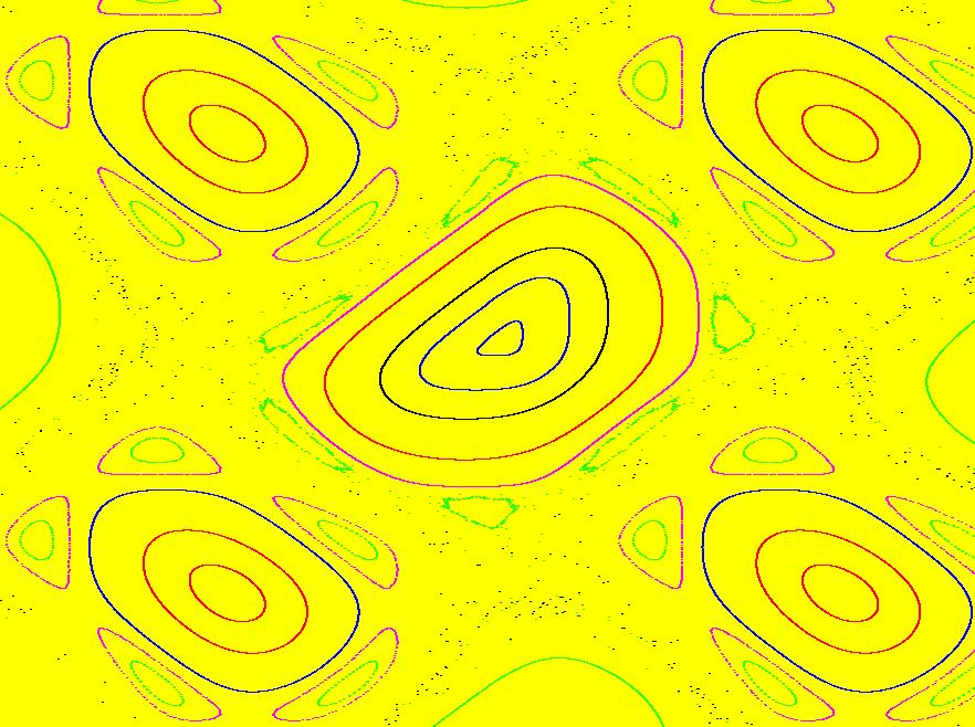
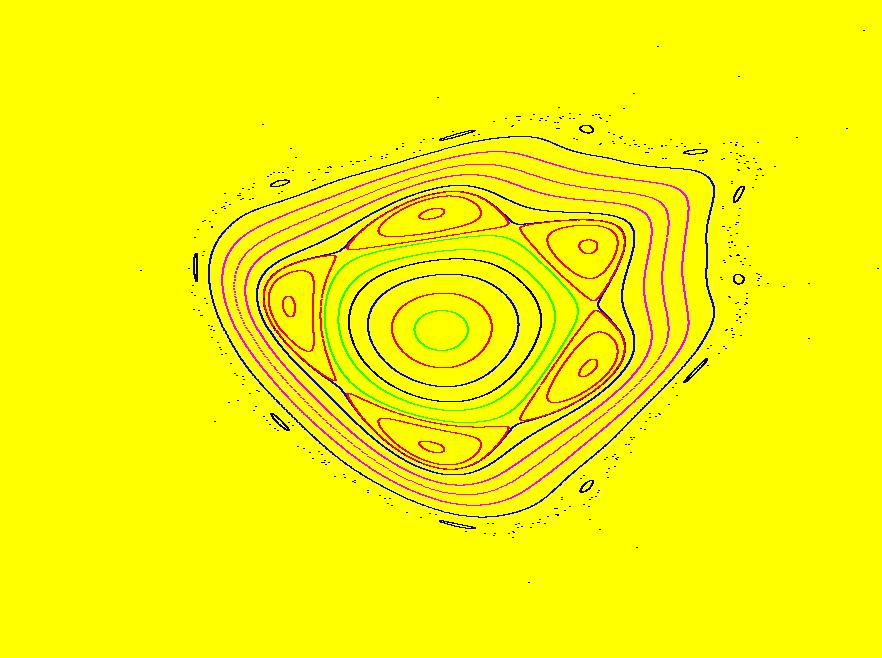
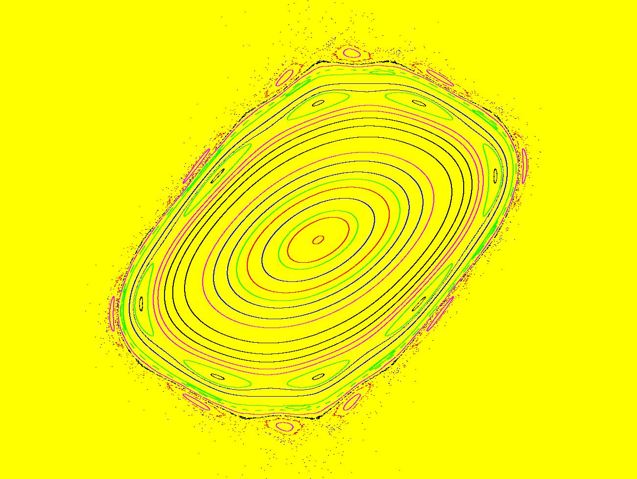
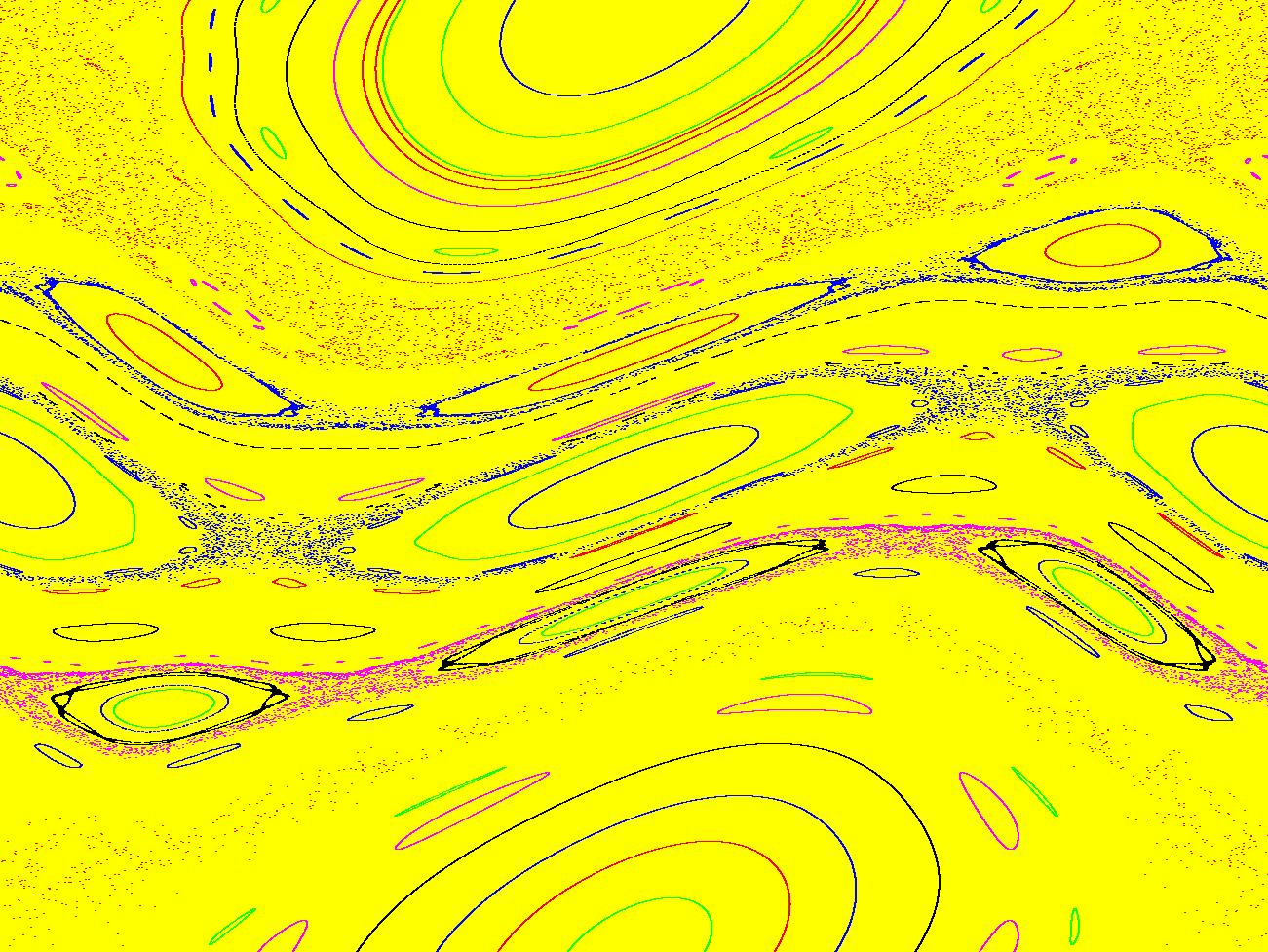
View/Sys/Gal: IMap "StandardMap: ( 3) IMap0011 (x+k*sin(y),x+y+k*sin(y)), k = 2.300; " in "MapExs." This iteration is defined by:
x <- x+k*sin(y),
y <- x+y+k*sin(y).
Parameters are:
k = 2.300;
There are periodic orbits at the "centers" of all of the "closed" curves (KAM islands).
Zoom out.
|
|
|
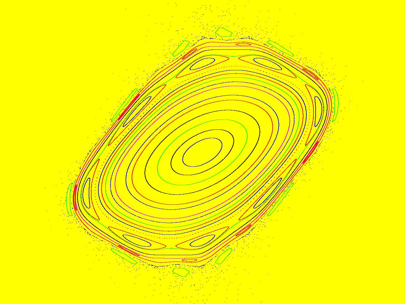
View/Sys/Gal: IMap "StandardMap: ( 4) IMap0011 (x+k*sin(y),x+y+k*sin(y)), k=.971635" in "MapExs." This iteration is defined by:
x <- x+k*sin(y),
y <- x+y+k*sin(y).
Parameters are:
k=.971635
|
|
|
View/Sys/Gal: IMap "StandardMap: ( 5) IMap0011 (x%k+p*sin(y%k),(x+y)%k+p*sin(y%k)), k=6.2831852; p=1" in "MapExs." This iteration is defined by:
x <- x%k+p*sin(y%k),
y <- (x+y)%k+p*sin(y%k).
Parameters are:
k=6.2831852; p=1
Wait for the image to be drawn.
Zoom in 3 times..
Zoom out again and vary p and k.
|
|
|
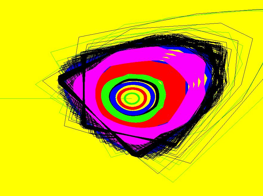
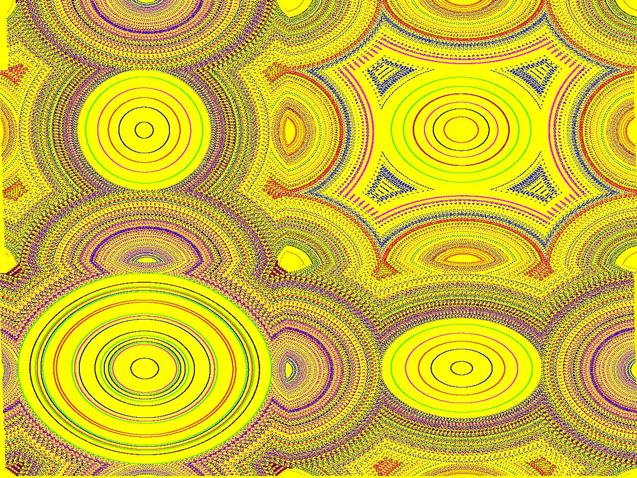
View/Sys/Gal: IMap "StandardMap: ( 6) IMap1110 (x%k+p*sin(y%k),(x+y)%k+p*sin(y%k)), k=6.2831852; p=1" in "MapExs." This iteration is defined by:
x <- x%k+p*sin(y%k),
y <- (x+y)%k+p*sin(y%k).
Parameters are:
k=6.2831852; p=1
The "dot" in the center of the image is a red period-6 orbit (you need to zoom in three times to see it). The blue orbit is a period-5 orbit. The green orbit is a period-8 orbit.
|
|
|
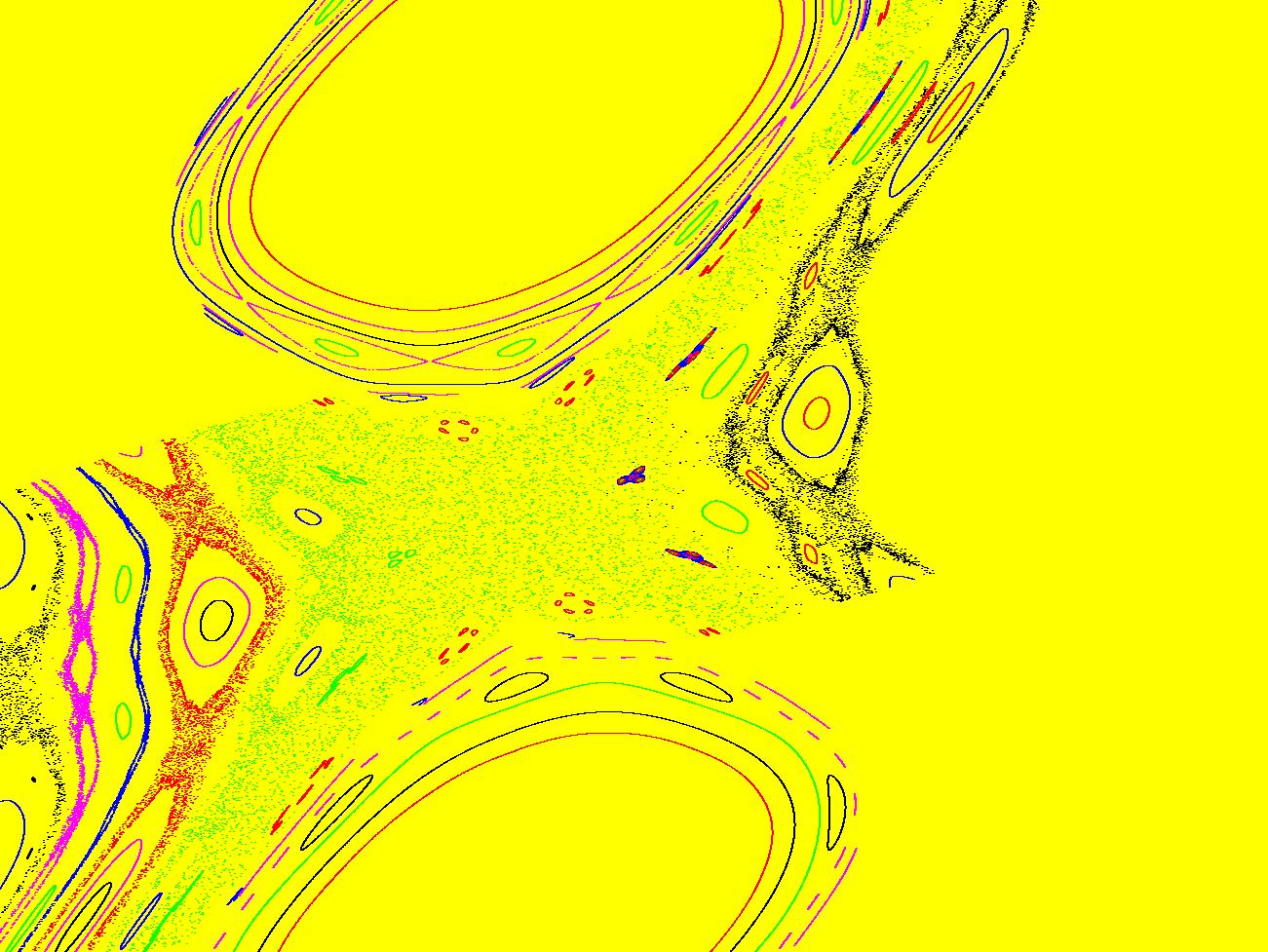
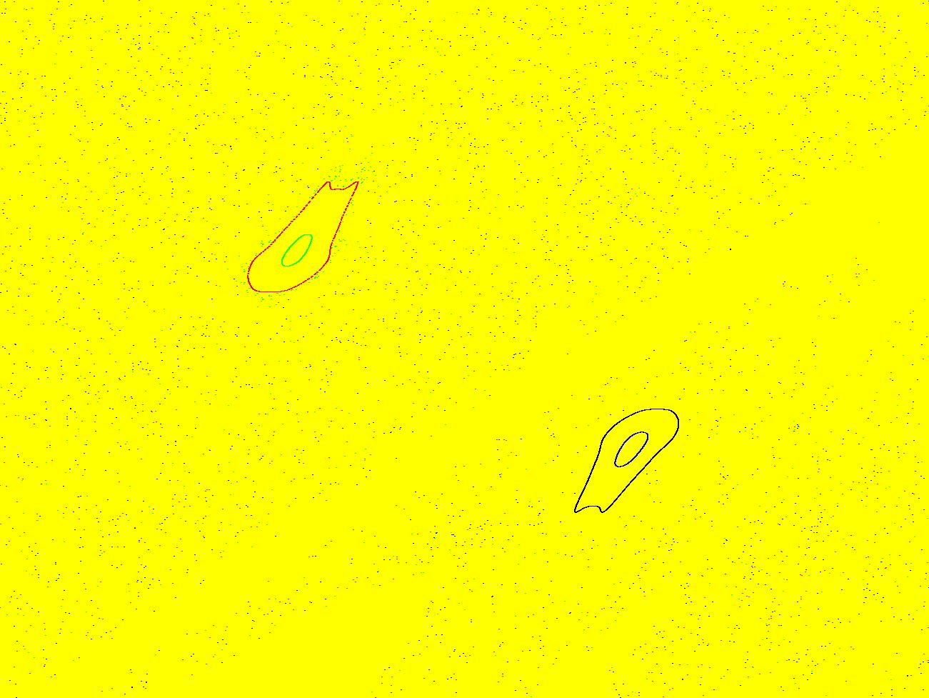
View/Sys/Gal: IMap "StandardMap: ( 7) IMap0011 (x%k+p*sin(y%k),(x+y)%k+p*sin(y%k)), k = -2.900; p = 2.100; " in "MapExs." This iteration is defined by:
x <- x%k+p*sin(y%k),
y <- (x+y)%k+p*sin(y%k).
Parameters are:
k = -2.900; p = 2.100;
Try k = -4.1 and p = -.6, 0, .3, .5, .9.
|
|
|
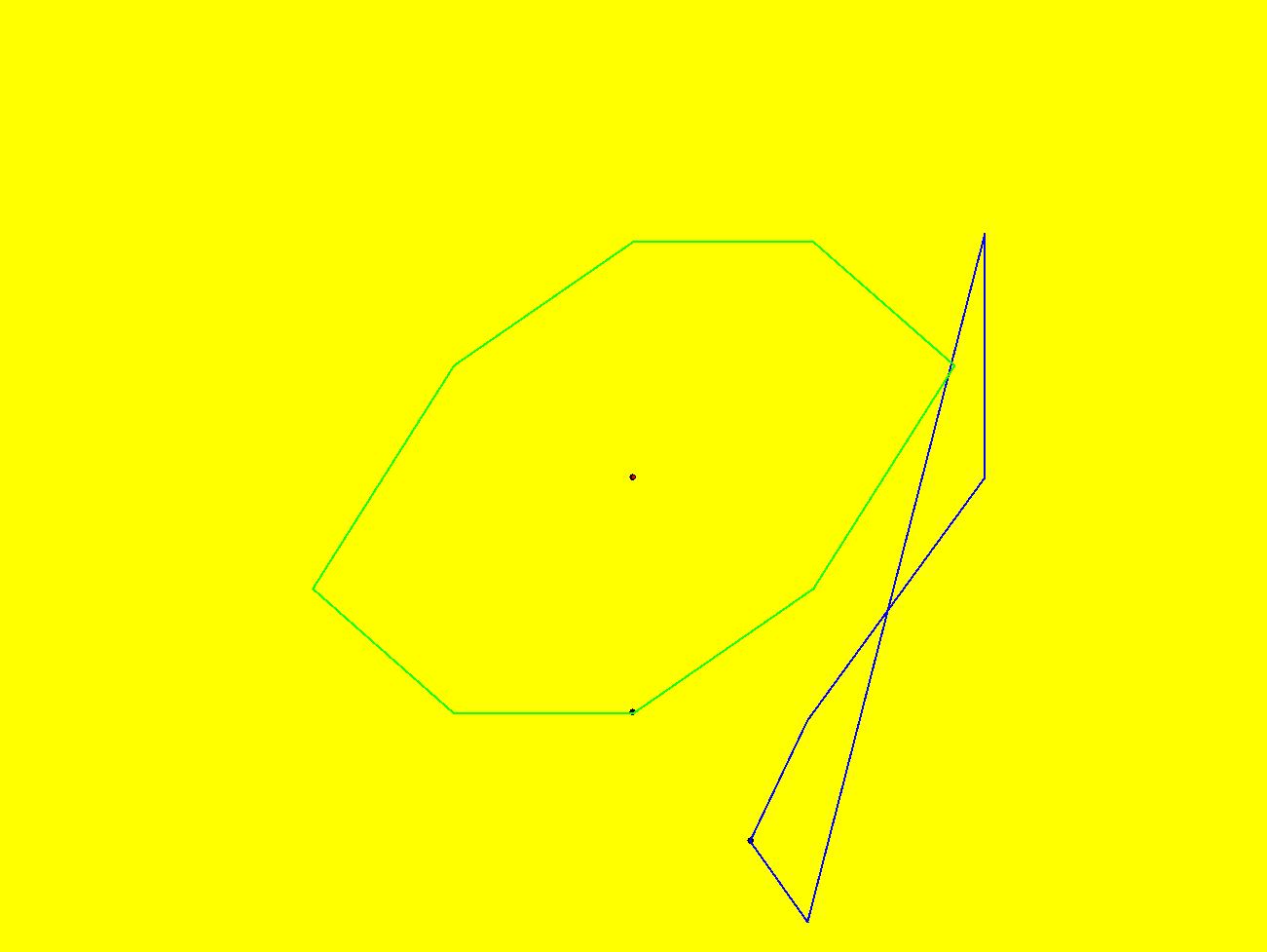
View/Sys/Gal: IMap "StandardMap: ( 8) IMap0011 ((x+y-k/6.283*sin(6.283*x))%6.283,(y-k/6.283*sin(6.283*x))%6.283), k = 2.00; " in "MapExs." This iteration is defined by:
x <- (x+y-k/6.283*sin(6.283*x))%6.283,
y <- (y-k/6.283*sin(6.283*x))%6.283.
Parameters are:
k = 2.00;
There is a lot more to this map. Zoom out and drag around to create more orbits.
There are period-5 orbits near
(x,y) = (-0.248889,-0.069495) and
(x,y) = (-0.248889,-0.247273).
Try to find them.
See the next system, "StandardMap: (9)..."
See gallery "PeriodicIMapOrbits."
|
|
|
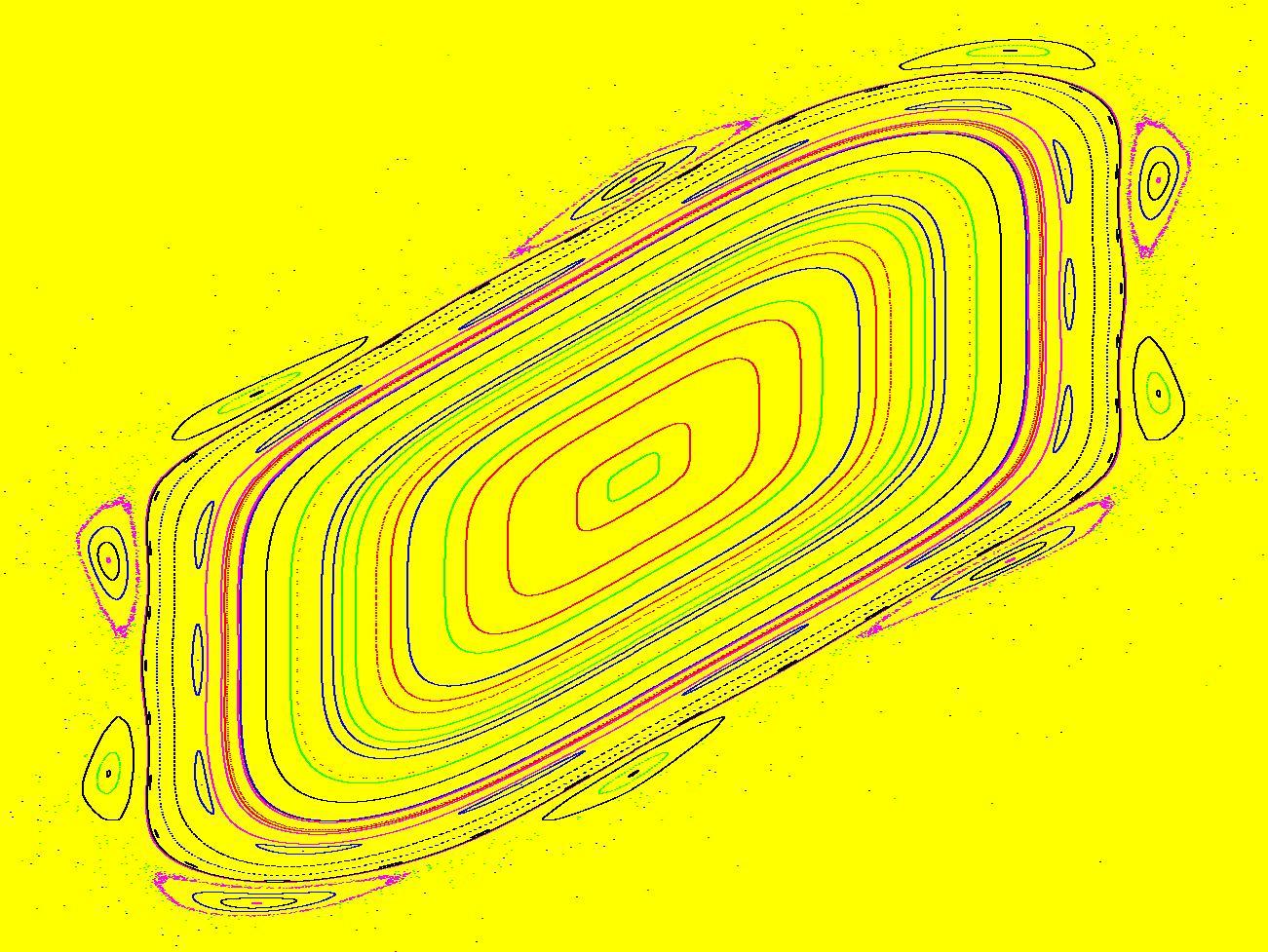
View/Sys/Gal: IMap "StandardMap: ( 9) IMap1100 ((x+y-k/6.283*sin(6.283*x))%6.283,(y-k/6.283*sin(6.283*x))%6.283), k = 2.00; " in "MapExs." This iteration is defined by:
x <- (x+y-k/6.283*sin(6.283*x))%6.283,
y <- (y-k/6.283*sin(6.283*x))%6.283.
Parameters are:
k = 2.00;
Two period-5 orbits are:
red: (-0.248287,-0.248287)
blue: (-0.248287,-0.070014).
Orbits near these two periodic orbits are also periodic with periods divisible by 5. Try to find a few.
The green orbit at (-0.206241,-0.153180) has period 14.
|
|
|
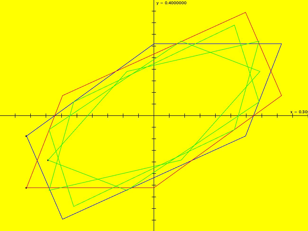
View/Sys/Gal: IMap "StandardMap: (10) IMap0011 Figure 1: k = 0.5" in "MapExs." This iteration is defined by:
x <- (x+(y+k*sin(x))%(2*pi))%(2*pi),
y <- (y+k*sin(x)).
Parameters are:
k=.5
Ref 1: Chirikov standard map.
Figures 1, 2 and 3 are the same as the corresponding figures in Ref 1. There is a period-2 orbit at ( π, π). To see it, start a Flow.
Ref 2: Kolmogorov-Arnold-Moser Theory.
Ref 2 is a general reference to KAM Theory.
Ref 3: The Standard Map
Ref 3 is another reference to the standard map.
|
|
|
View/Sys/Gal: IMap "StandardMap: (11) IMap0011 Figure 3: k = 0.971635" in "MapExs." This iteration is defined by:
x <- (x+(y+k*sin(x))%(2*pi))%(2*pi),
y <- (y+k*sin(x)).
Parameters are:
k=.971635
|
|
|
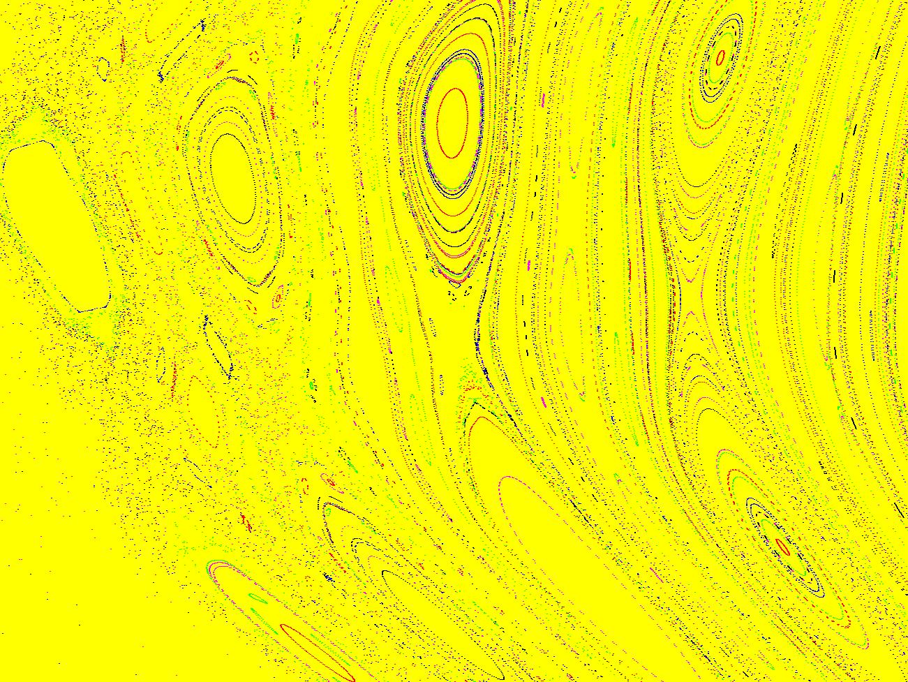
View/Sys/Gal: IMap "StandardMap: (12) IMap0011 Figure 3: k = 5" in "MapExs." This iteration is defined by:
x <- (x+(y+k*sin(x))%(2*pi))%(2*pi),
y <- (y+k*sin(x)).
Parameters are:
k = 5.000;
|
|
|
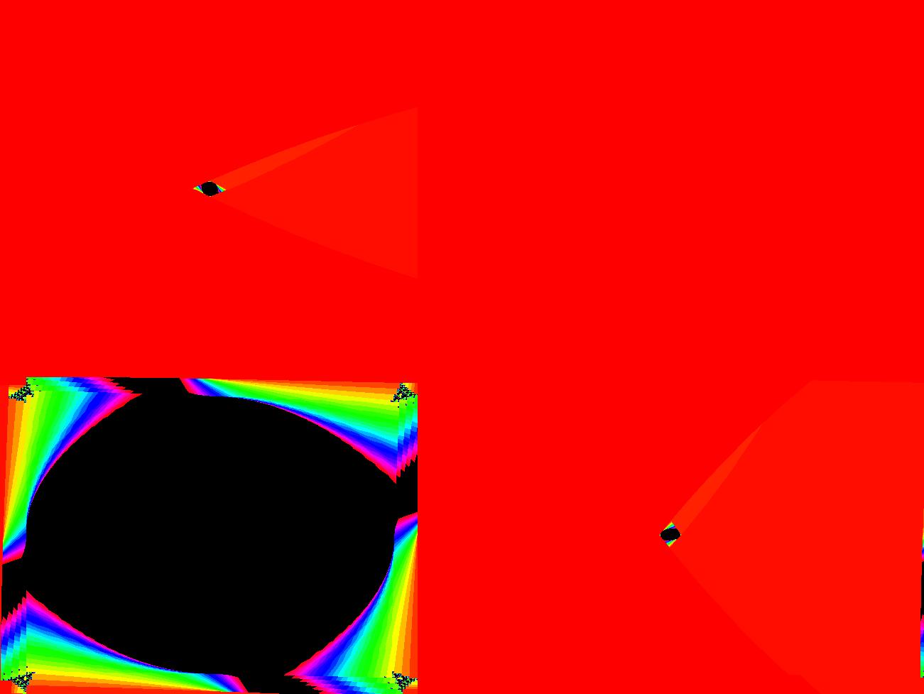
View/Sys/Gal: EMap "StandardMap: (13) EMap" in "MapExs." This iteration is defined by:
x <- x%k+p*sin(y%k),
y <- (x+y)%k+p*sin(y%k).
Parameters are:
k = 6.300; p = .900;
Try some other color tables.
|
|
|
View/Sys/Gal: EMap "StandardMap: (14) EMap 2" in "MapExs." This iteration is defined by:
x <- x%k+p*sin(y%k),
y <- (x+y)%k+p*sin(y%k).
Parameters are:
k = 6.300; p = .900;
Try some other color tables.
|
|
|
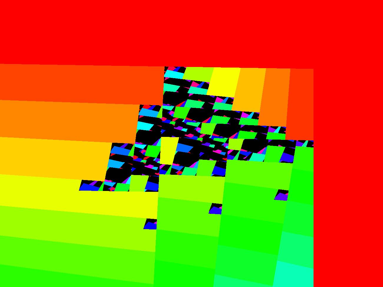
View/Sys/Gal: EMap "StandardMap: (15 EMap 3" in "MapExs." This iteration is defined by:
x <- (1+s*.1)*(x%k+p*sin(y%k)),
y <- (1+s*.1)*((x+y)%k+p*sin(y%k)).
Parameters are:
k = 5.000; p = .240; s = .420;
Increase s to decrease the black.
|
|
|
View/Sys/Gal: EMap "StandardMap: (16) EMap 4" in "MapExs." This iteration is defined by:
x <- (1+s*.1)*(x%k+p*sin(y%k)),
y <- (1+s*.1)*((x+y)%k+p*sin(y%k)).
Parameters are:
k = 5.000; p = .240; s = .420;
|
|
|
View/Sys/Gal: EMap "StandardMap: (17) EMap 5" in "MapExs." This iteration is defined by:
x <- (1+s*.1)*(x%k+p*sin(y%k)),
y <- (1+s*.1)*((x+y)%k+p*sin(y%k)).
Parameters are:
k = 5.000; p = .240; s = .420;
|
