Click on an image to go directly to a system or scroll to see the systems in this gallery.
 |
 |
 |
 |
 |
 |
 |
 |
 |
 |
 |
 |
 |
 |
 |
 |
 |
 |
 |
 |
 |
 |
 |
 |
 |
 |
 |
 |
 |
 |
 |
 |
 |
 |
 |
 |
 |
 |
 |
| OdeFactory Images and Annotations | |
|
|
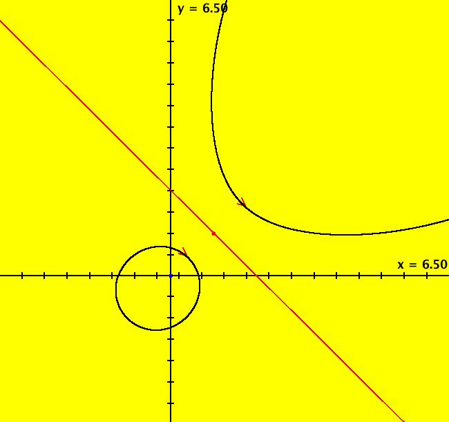
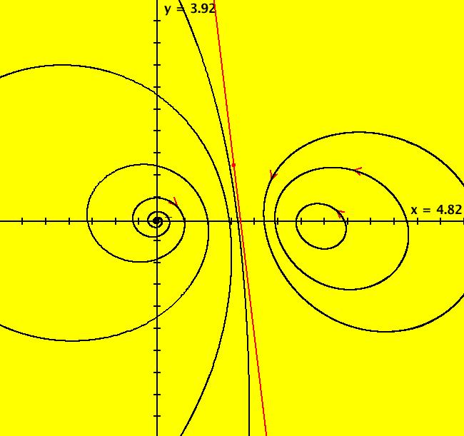
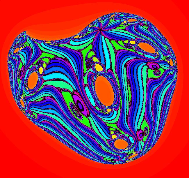
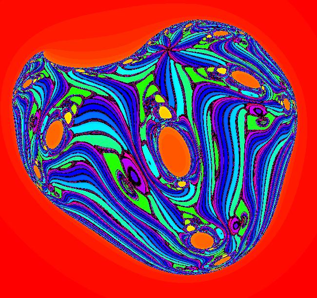
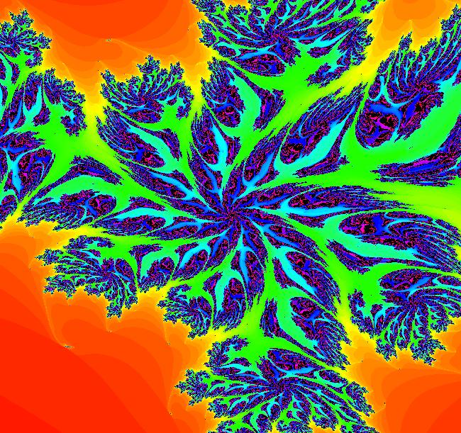
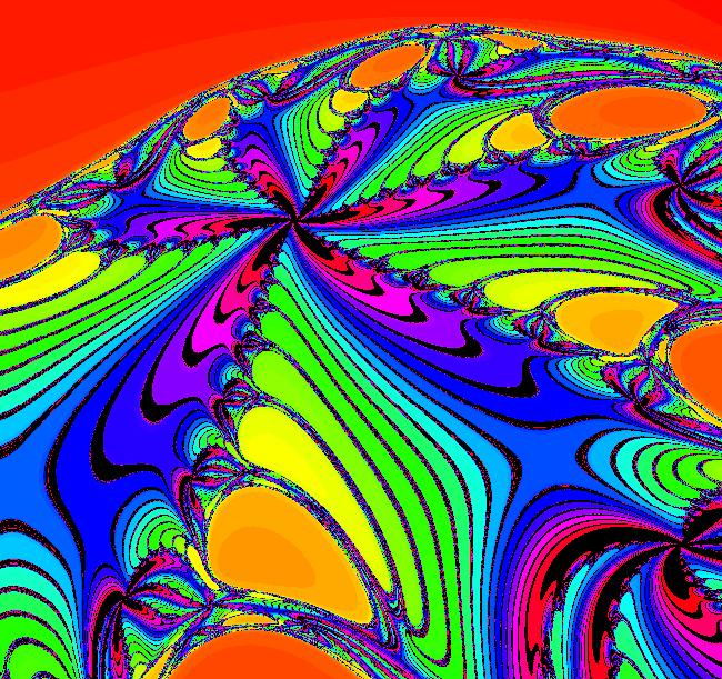
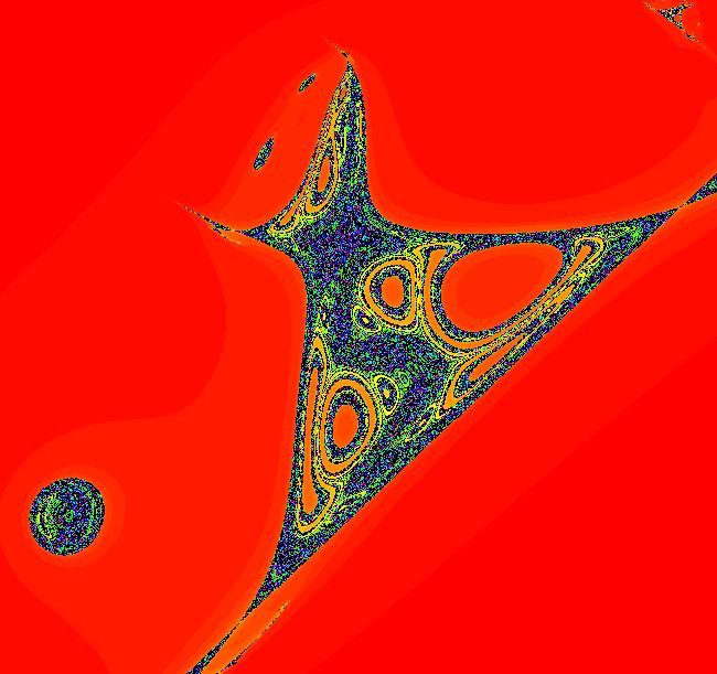
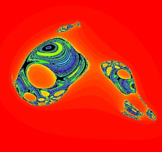
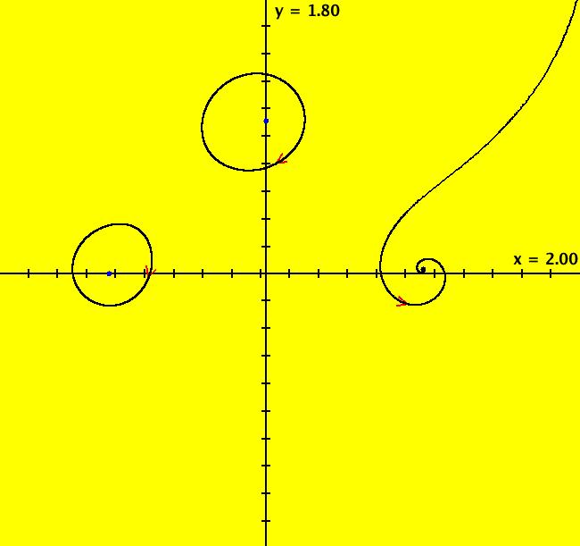
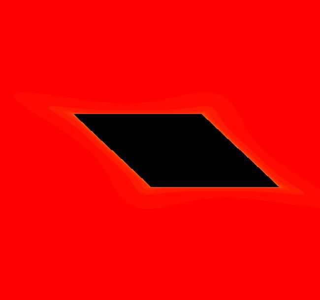
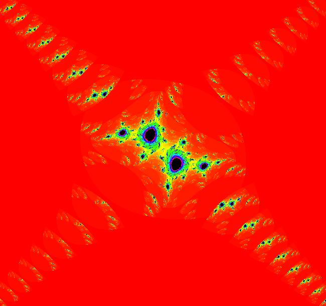
View/Sys/Gal: EMap "AGF: 1 complex line and a real line, EMap" in "AGFractals." This AGF is generated by the lines: L[1]: (x-1)+(y-1) = 0, m = -1, λ1 = 1 I[1]: x+i*y = 0, λ1 = i The degree of the RHS of the system is: 2. Shift-click on the complex line and on the real line to open slider-based parameter controllers. Vary the 12 control parameters to find interesting EMap variations. In general a 2D polynomial system has 2*(3+2+1) = 12 control parameters. The 2D Mandelbot system, z <- z^2+c, has only 2 control parameters. Image 1: Ode view. Image 2: EMap view.
|
|
|
View/Sys/Gal: EMap "AGF: 1 complex line and a real line, ver 2, EMap" in "AGFractals." This AGF is generated by the lines: L[1]: (x-1.2)+0.10753*(y-1) = 0, m = -9.3, λ1 = 0.9 I[1]: x+i*y = 0, λ1 = (0.14+i) The degree of the RHS of the system is: 2. Image 1: Ode view. Image 2: EMap view.
|
|
|
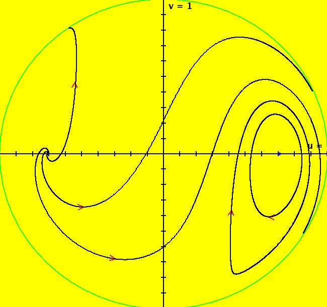
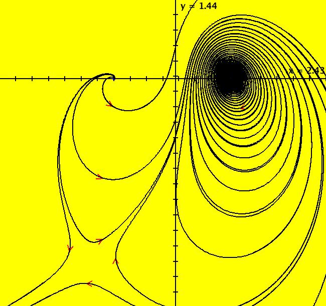
View/Sys/Gal: EMap "AGF: 2 complex lines, EMap" in "AGFractals." This AGF is generated by the lines: I[1]: (x-1)+i*y = 0, λ1 = i I[2]: (x+1)+i*y = 0, λ2 = (1-i) The degree of the RHS of the system is: 3. Image 1: Ode R2+ view. Image 2: EMap view.
|
|
|
View/Sys/Gal: EMap "AGF: 2 complex lines, in dx/dt, dy/dt form, EMap" in "AGFractals." This system of odes is defined by: dx/dt = (1-x^2+x^3+y^2+x*(-1+4*y+y^2))/4, dy/dt = (x^2*(-2+y)-2*x*y+(2+y)*(1+y^2))/4. It is the same as the previous AGF but it is has been rewritten in the traditional dx/dt, dy/dt form. Image 1: EMap view.
|
|
|
View/Sys/Gal: EMap "AGF: 2 complex lines, ver 2, EMap" in "AGFractals." This system is the result of adjusting the 8 parameters for I[1] in system: AGF: 2 complex lines, EMap The AGF is generated by the lines: I[1]: (1.1+0.01*i)*(x-0.9)+(0.12+0.8*i)*(y-0.01) = 0, λ1 = (0.03+1.2*i) I[2]: (x+1)+i*y = 0, λ2 = (1-i) The degree of the RHS of the system is: 3. Image 1: Ode view. Image 2: EMap view.
|
|
|
View/Sys/Gal: EMap "AGF: 2 complex lines, ver 3, EMap" in "AGFractals." This AGF is generated by the lines: I[1]: 1.43*(x-1)+1.2*i*y = 0, λ1 = (1.3-0.4*i) I[2]: 1.1*(x+1)+i*y = 0, λ2 = (-1.56+0.99*i) The degree of the RHS of the system is: 3. Image 1: Ode view. Image 2: EMap view.
|
|
|
View/Sys/Gal: EMap "AGF: 2 complex lines, ver 4, EMap" in "AGFractals." This AGF is generated by the lines: I[1]: 1.43*(x-1)+1.2*i*y = 0, λ1 = (1.3-0.4*i) I[2]: 1.1*(x+1)+i*y = 0, λ2 = (-1.56+0.99*i) The degree of the RHS of the system is: 3. Image 1: Ode R2+ view. Image 2: EMap view.
|
|
|
View/Sys/Gal: EMap "AGF: 2 complex lines, ver 5, EMap" in "AGFractals." This AGF is generated by the lines: I[1]: (1.1+0.01*i)*(x-1)+(0.01+0.8*i)*y = 0, λ1 = (0.01+1.1*i) I[2]: (x+1.4)+(-0.01+0.7*i)*y = 0, λ2 = (1-1.1*i) The degree of the RHS of the system is: 3. Image 1: Ode R2+ view. Image 2: EMap view.
|
|
|
View/Sys/Gal: EMap "AGF: 2 complex lines, ver 6, EMap" in "AGFractals." This AGF is generated by the lines: I[1]: (x-1)+i*y = 0, λ1 = (0.005+i) I[2]: (x+1)+i*y = 0, λ2 = (1-i) The degree of the RHS of the system is: 3. Image 1: Ode R2+ view. Image 2: EMap view.
|
|
|
View/Sys/Gal: EMap "AGF: 2 complex lines, ver 7, EMap" in "AGFractals." This AGF is generated by the lines: I[1]: 1.4*(x-1)+1.2*i*y = 0, λ1 = (1.9-0.07*i) I[2]: 1.1*(x+1)+i*y = 0, λ2 = (-1.56+0.99*i) The degree of the RHS of the system is: 3. Image 1: Ode view. Image 2: EMap view.
|
|
|
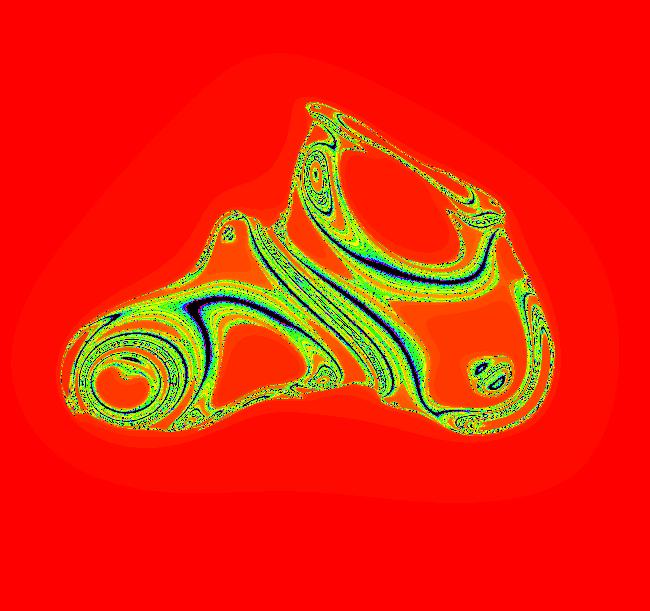
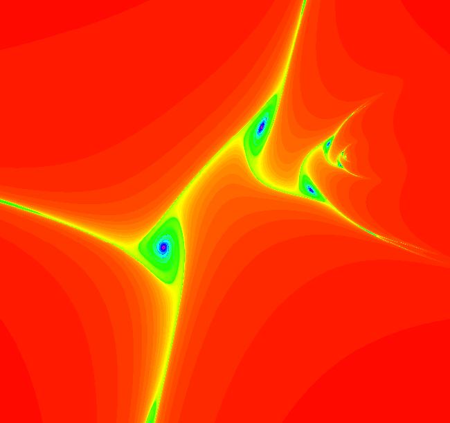
View/Sys/Gal: EMap "AGF: 3 complex lines" in "AGFractals." This AGF is generated by the lines: I[1]: x+i*(y-1) = 0, λ1 = i I[2]: (x-1)+i*y = 0, λ2 = i I[3]: (x+1)+i*y = 0, λ3 = i The degree of the RHS of the system is: 5. This is an interesting Ode but it is not so interesting in the IMap or EMap views. Image 1: Ode view. Image 2: EMap view.
|
|
|
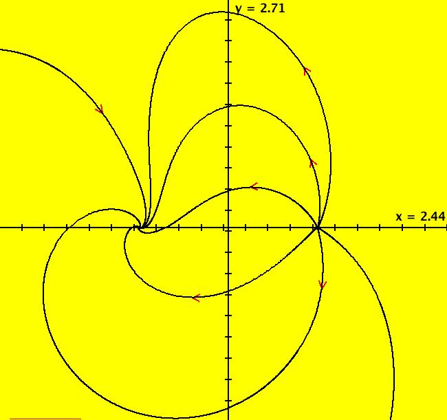
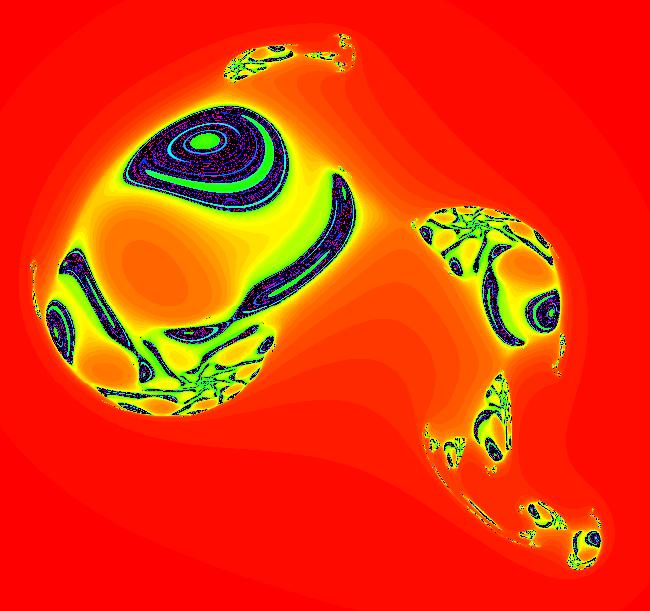
View/Sys/Gal: EMap "AGF: 3 complex lines, 1 real line" in "AGFractals." This AGF is generated by the lines: L[1]: x-y = 0, m = 1, λ1 = 0.01 I[1]: x+i*(y-1) = 0, λ1 = (-0.1+i) I[2]: (x-1)+i*y = 0, λ2 = (-0.1+i) I[3]: (x+1)+i*y = 0, λ3 = (0.1+i) The degree of the RHS of the system is: 6. Another interesting Ode. Image 1: Ode view. Image 2: EMap view.
|
|
|
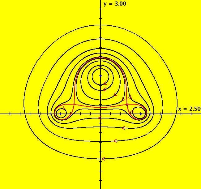
View/Sys/Gal: EMap "AGF: 3 complex lines, 1 real line, ver 2" in "AGFractals." This AGF is generated by the lines: L[1]: x-y = 0, m = 1, λ1 = -0.01 I[1]: x+i*(y-1) = 0, λ1 = (-0.1+i) I[2]: (1-0.3*i)*(x+0.3)+i*(y-0.82) = 0, λ2 = (-0.1-1.1*i) I[3]: (x+1)+i*y = 0, λ3 = (0.1+i) The degree of the RHS of the system is: 6. An interesting Ode and EMap. Image 1: Ode view. Image 2: EMap view.
|
|
|
View/Sys/Gal: EMap "AGF: 3 complex lines, ver 2, EMap" in "AGFractals." This AGF is generated by the lines: I[1]: x+i*(y-1) = 0, λ1 = i I[2]: (-2+0.5*i)*(x-1)+(0.3+2.01*i)*y = 0, λ2 = (-0.15+1.4*i) I[3]: (x+1)+i*y = 0, λ3 = i The degree of the RHS of the system is: 5. Sort of an interesting Ode but a more interesting EMap. Image 1: Ode view. Image 2: EMap view.
|
|
|
View/Sys/Gal: EMap "AGF: 3 complex lines, ver 3, EMap" in "AGFractals." This AGF is generated by the lines: I[1]: (1.0001+1.2*i)*(x-0.001)+(0.5001+2*i)*(y-1.0001) = 0, λ1 = (-2.06-0.45*i) I[2]: (x-1)+i*y = 0, λ2 = i I[3]: (x+1)+i*y = 0, λ3 = i The degree of the RHS of the system is: 5. Image 1: Ode view. Image 2: EMap view.
|
|
|
View/Sys/Gal: EMap "AGF: 3 complex lines, ver 4, EMap" in "AGFractals." This AGF is generated by the lines: I[1]: x+i*(y-1) = 0, λ1 = i I[2]: (1-0.01*i)*(x-1)+(-0.04+i)*(y-0.03) = 0, λ2 = (-0.51-1.4*i) I[3]: (x+1)+i*y = 0, λ3 = i The degree of the RHS of the system is: 5. Image 1: Ode view. Image 2: EMap view.
|
|
|
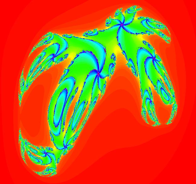
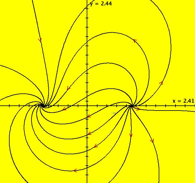
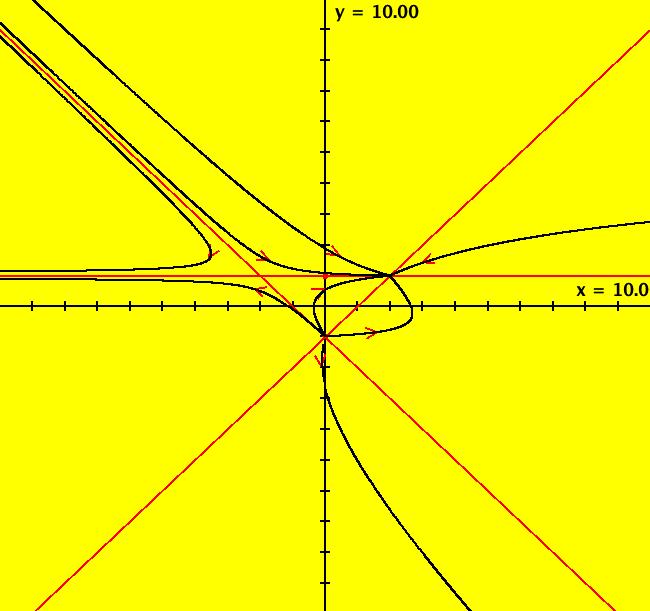
View/Sys/Gal: EMap "AGF: 3 real lines" in "AGFractals." This AGF is generated by the lines: L[1]: x-(y+1) = 0, m = 1, λ1 = 1 L[2]: x+(y+1) = 0, m = -1, λ2 = 1 L[3]: (y-1) = 0, m = 0, λ3 = 1 The degree of the RHS of the system is: 2. Image 1: Ode view. Image 2: EMap view.
|
|
|
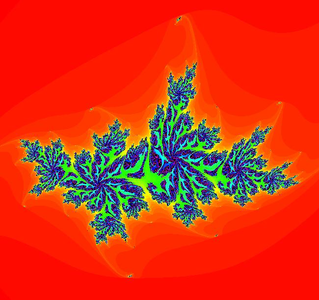
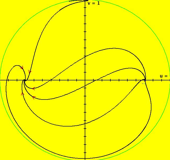
View/Sys/Gal: EMap "AGF: 3 real lines, ver 2, EMap" in "AGFractals." This AGF is generated by the lines: L[1]: x-0.2381*(y+1) = 0, m = 4.2, λ1 = 1.2 L[2]: x+(y+1) = 0, m = -1, λ2 = -5 L[3]: (y-1) = 0, m = 0, λ3 = -1 The degree of the RHS of the system is: 2. Image 1: Ode R2+ view. Image 2: EMap view.
|
|
|
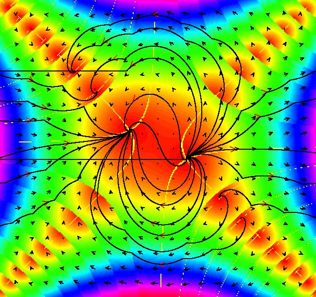
View/Sys/Gal: EMap "AGFv: variation 1 of star-in & star-out, EMap" in "AGFractals." This system of odes is defined by the equations: dx/dt = b*x^2-y^2+p, dy/dt = a*x*y%c+q Parameters are: p = -.70; q = 1.00; a = 1.00; b = .30; c = 6.70; Image 1: Ode view with colored V fld on. Image 2: EMap view.
|
|
|
View/Sys/Gal: EMap "AGFv: variation 2 of star-in & star-out, EMap" in "AGFractals." This system of odes is defined by the equations: dx/dt = x^2-y^2+p, dy/dt = 2*x%y+q Parameters are: p = -.65; q = 1.00; Image 1: Ode view with colored V fld on. Image 2: EMap view.
|