Click on an image to go directly to a system or scroll to see the systems in this gallery.

OdeFactory Images and Annotations

An OdeFactory Slide Show
Click on a slide to zoom in.
Click "video" to see a video.

View/Sys/Gal: Ode " AGFs and Escape-time Maps" in "AGFEMapExsB."
Range: (vMax,vMin) = (5.000,-5.000), (hMin,hMax) = (-5.000,5.000)
VFld: (0)
-------- AGFs and Eacape-time Maps --------
AGF is short for "algebraically generated flow." An AGF is a 2D autonomous system of odes.
AGFs have polynomial vector fields. The vector fields are constructed in OdeFactory by selecting real and/or complex linear generators using the "Define an AGF" window.
The original idea, from 1973, was to create global phase portraits with specific local topological features.
Real generators, called real lines, generate straight line separatrices.
Complex generators, called complex lines, generate fixed points corresponding to centers, spirals and stars.
The combination of real and complex lines spawn additional fixed points that can themselves be centers, saddles or spirals.
The EMap view of AGFs are often fractals
Fractals were first studied in 1978 when it became possible to use computers to produce escape-time maps.
When I retired in 2000 from the CS Department at UW Madison I began writing OdeFactory to verify some of the hand computations relating to AGFs that I did in the 70s. As an afterthought, I added the IMap and EMap algorithms to the program to study iteration maps and escape-time maps. It turned out that the Mandelbrot map, z <- z^2+c, can be generated from two complex lines.
This gallery shows several other AGFs that generate new fractals in the EMap view.
For more details, select "AGFs" on the Help menu.

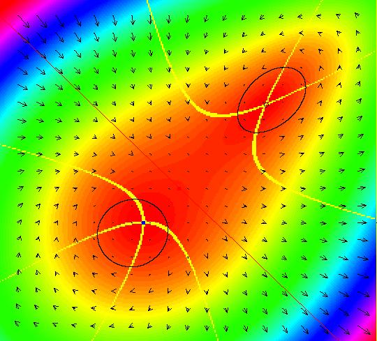
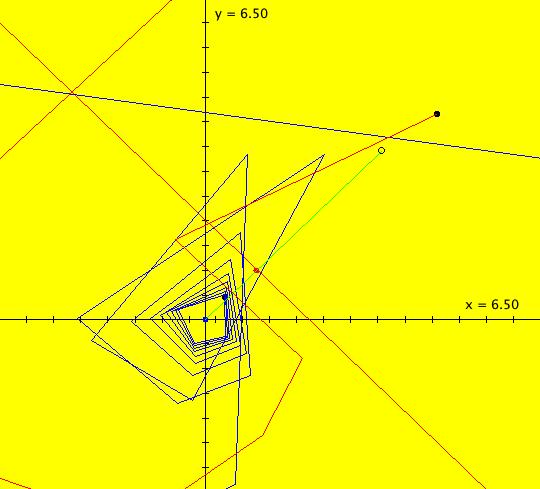
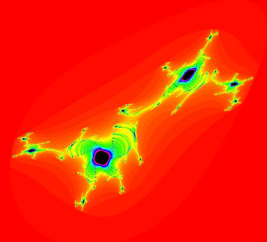
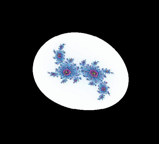
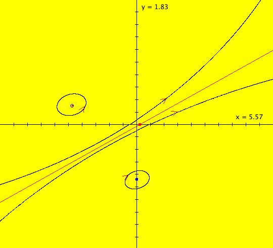
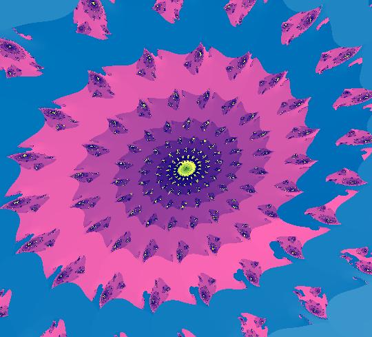
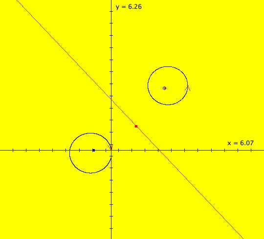
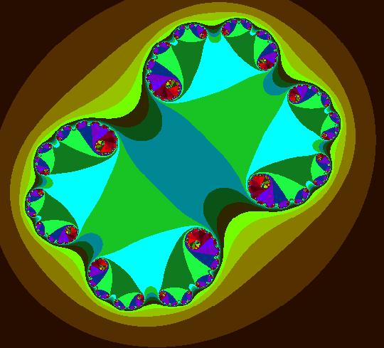
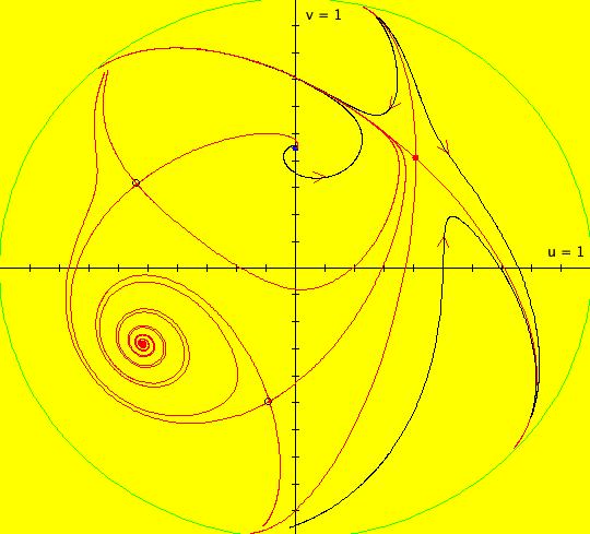
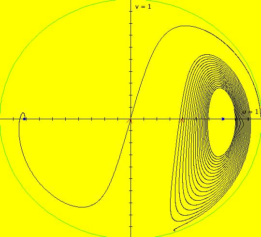
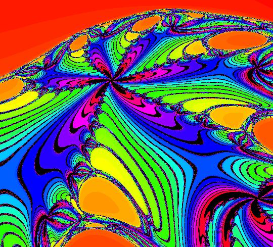
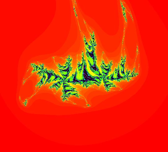
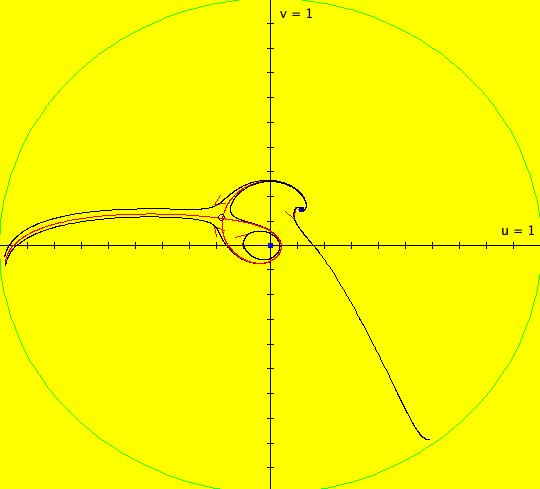
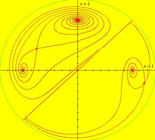
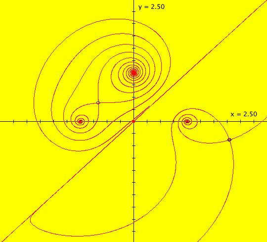
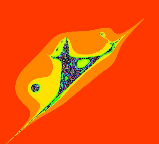
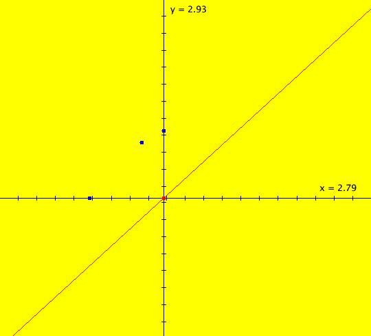
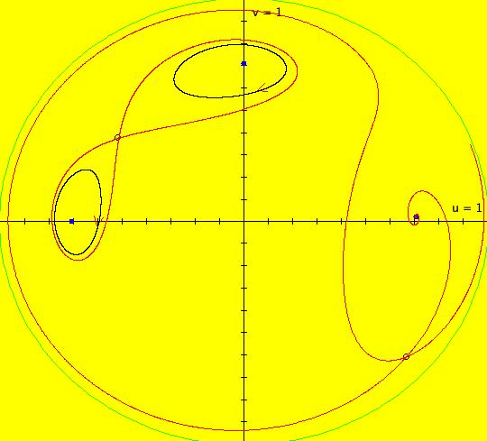
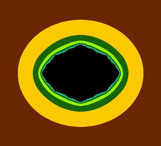
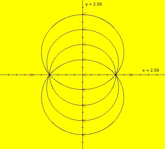
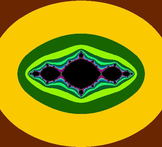
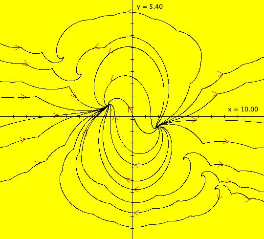
View/Sys/Gal: EMap "AGF: 1 complex line and a real line, EMap" in "AGFEMapExsB."
Range: (vMax,vMin) = (6.500,-3.500), (hMin,hMax) = (-4.000,6.500)
VFld: AGF
This AGF is generated by the lines:
L[1]: (x-1)+(y-1) = 0, m = -1, λ₁ = 1
I[1]: x+i*y = 0, λ₁ = i
The degree of the RHS of the system is: 2.
In traditional form the system is:
dx/dt = 0.3535*x^2+
        (0.999698-0.499849*x)*y-0.146349*y^2
dy/dt = x*(-0.999698+0.146349*x+0.499849*y)
        -0.3535*y^2
Image 1: the colored vector field. The blue dot is the complex line I[1], the red line is the real line L[1]. The yellow curves are nullclines.
The ode system has two fixed points at the crossing points of the nullclines, one at (0,0) and one at (3.409594,3.414141). The red line is a straight line trajectory and all other trajectories are cycles.
Image 2: the IMap view. The green orbit, starting at (3.409594,3.414141), goes to the fixed point (0,0). All other orbits go to infinity.
Image 3: the EMap view. In the EMap we get a fractal.
In general a 2D polynomial system in the dx/dt, dy/dt form has 2*(3+2+1) = 12 control parameters. The 2D Mandelbrot system, z <- z^2+c, has only 2 control parameters. The reduction in the number of parameters is due to the symmetry of the Mandelbrot system. See OdeFactory gallery AGFs&Mandelbrot for details.
Shift-click on the complex line and on the real line to open slider-based parameter controllers. Vary the 12 control parameters to find interesting EMap variations.

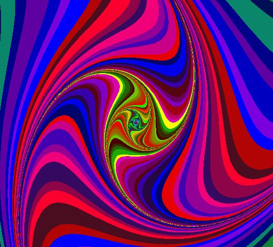
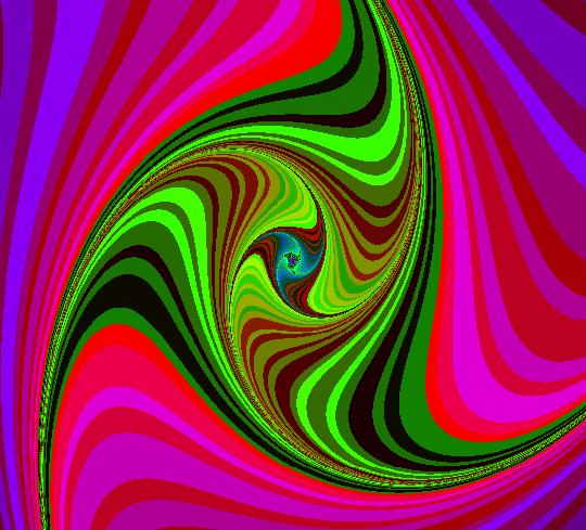
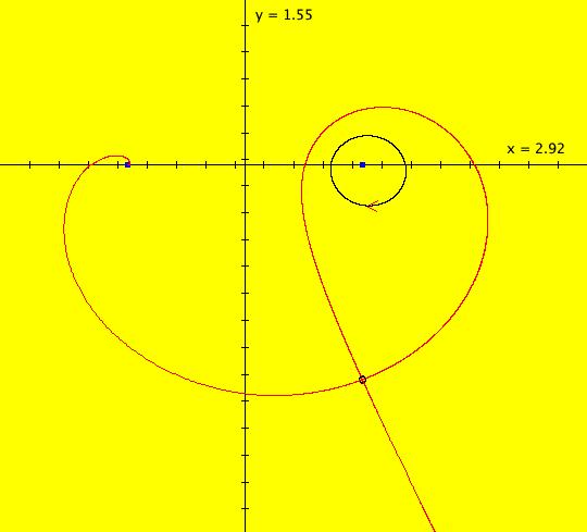
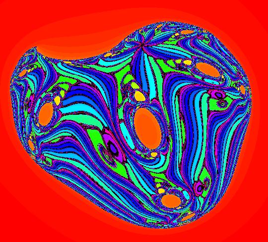
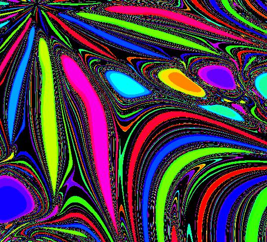
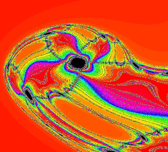
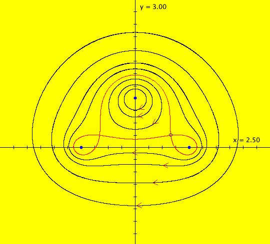
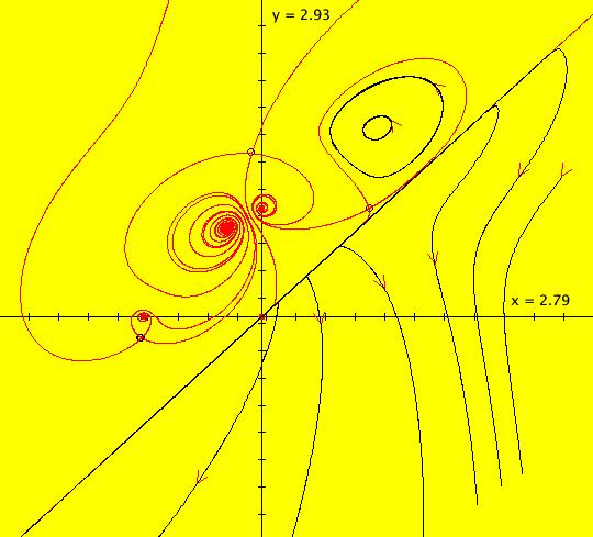
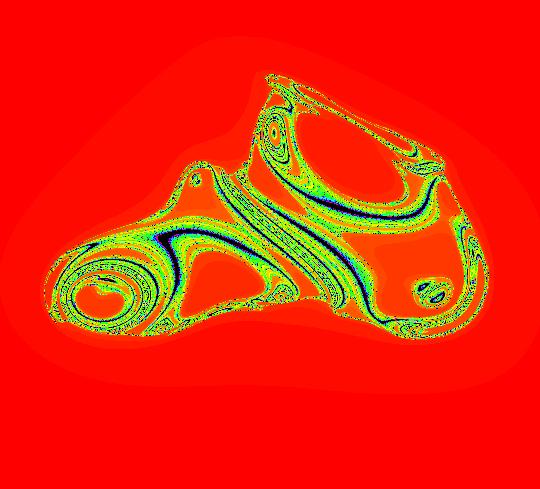
View/Sys/Gal: EMap "AGF: 1 complex line and a real line, ver 2, EMapMaxCT3" in "AGFEMapExsB."
Range: (vMax,vMin) = (7.791,-7.698), (hMin,hMax) = (-6.137,8.477)
VFld: AGF
This AGF is generated by the lines:
L[1]: (x-1.2)+0.10753*(y-1) = 0, m = -9.3, λ₁ = 0.9
I[1]: x+i*y = 0, λ₁ = (0.14+i)
The degree of the RHS of the system is: 2.
Image 1: Ode view. I[1] is a cw spiral out, L[1] is a straight line separatrix with flow downward.
Image 2: EMap view.

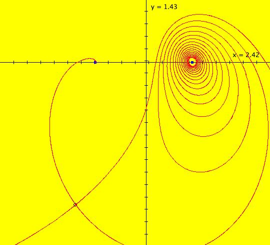
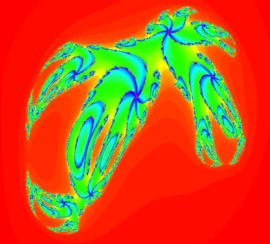
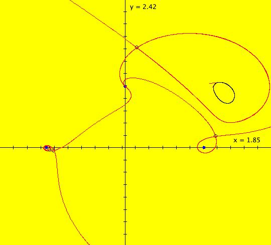
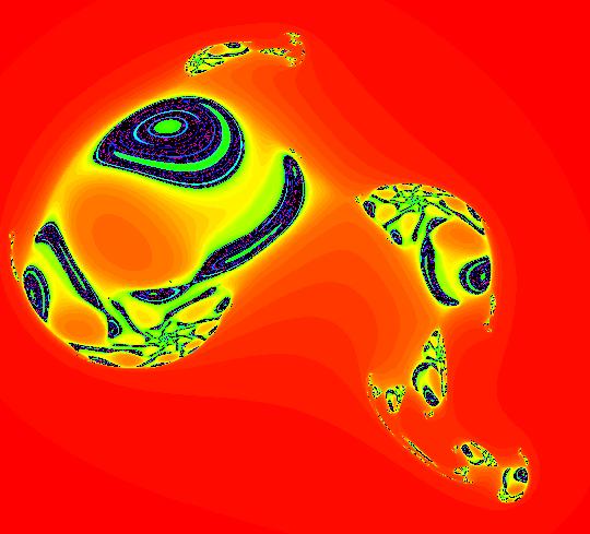
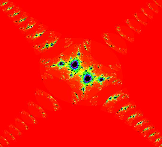
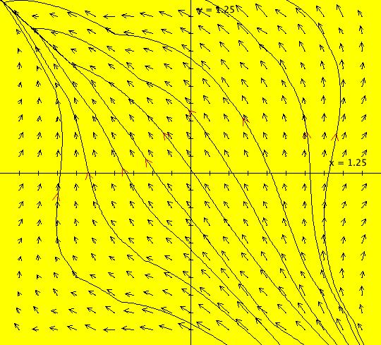
View/Sys/Gal: EMap "AGF: 1 complex line and a real line, ver 3, EMapMaxCT1" in "AGFEMapExsB."
Range: (vMax,vMin) = (1.831,-1.831), (hMin,hMax) = (-5.573,5.573)
VFld: AGF
This AGF is generated by the lines:
L[1]: (x-0.13)-5*y = 0, m = 0.2, λ₁ = -1
I[1]: (1-0.26*i)*(x+0.01)+(0.13+3.9*i)*(y+0.8) = 0, λ₁ = 0.6*i
The degree of the RHS of the system is: 2.
There is a spontaneous critical point at
        (x,y) = (-2.629256,0.279010).
Image 1: Ode view.
Image 2: EMap view.

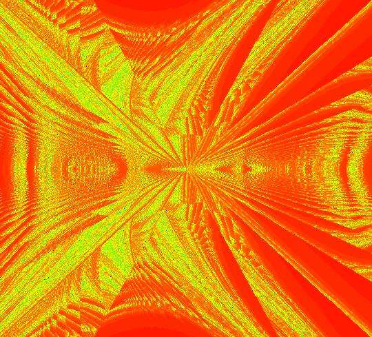
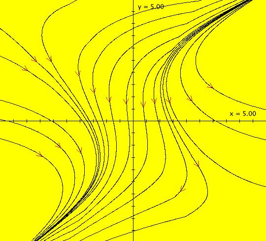
View/Sys/Gal: EMap "AGF: 1 complex line and a real line, ver 4, EMapMaxCT3" in "AGFEMapExsB."
Range: (vMax,vMin) = (0.846,0.659), (hMin,hMax) = (1.366,1.937)
VFld: AGF
This AGF is generated by the lines:
L[1]: (x-0.11)-5*y = 0, m = 0.2, λ₁ = -1
I[1]: (1-0.26*i)*(x+0.01)+
        (0.13+3.9*i)*(y+0.8) = 0, λ₁ = 0.6*i
The degree of the RHS of the system is: 2.
Image 1: Ode R2+ view.
Image 2: EMap view.

View/Sys/Gal: EMap "AGF: 1 complex line and a real line, ver 5, EMapMaxCT1" in "AGFEMapExsB."
Range: (vMax,vMin) = (6.255,-3.745), (hMin,hMax) = (-4.427,6.073)
VFld: AGF
This AGF is generated by the lines:
L[1]: (x-1)+0.909091*(y-1) = 0, m = -1.1, λ₁ = 1
I[1]: (x+0.7)+i*y = 0, λ₁ = i
The degree of the RHS of the system is: 2.
Image 1: Ode view.
Image 2: EMap view.
This is almost a Mandelbrot fractal. If you zoom in several times you can see that the symmetry is not exact.

View/Sys/Gal: EMap "AGF: 1 complex line and a real line, ver 6, EMapCT2" in "AGFEMapExsB."
Range: (vMax,vMin) = (5.000,-5.000), (hMin,hMax) = (-5.250,5.250)
VFld: AGF
This AGF is generated by the lines:
L[1]: x+0.909091*y = 0, m = -1.1, λ₁ = 1
I[1]: (x+1.678044)+i*(y+1) = 0, λ₁ = i
The degree of the RHS of the system is: 2.
Image 1: Ode view;
Image 2: EMap view.

View/Sys/Gal: EMap "AGF: 2 complex lines and two real lines, EMapMaxCT2" in "AGFEMapExsB."
Range: (vMax,vMin) = (0.224,0.224), (hMin,hMax) = (0.236,0.236)
VFld: AGF
This AGF is generated by the lines:
L[1]: (x-0.5)+(y-0.5) = 0, m = -1, λ₁ = 1
L[2]: (x-0.5)-0.196078*(y-0.5) = 0, m = 5.1, λ₂ = -1.8
I[1]: (-8.6-0.88*i)*(x+0.64)+(0.97+10*i)*(y+0.35) = 0, λ₁ = (0.98-9.8*i)
I[2]: x+i*(y-0.5) = 0, λ₂ = (1-i)
The degree of the RHS of the system is: 5.
The ode view has 2 spontaneous fixed points. They are saddles at about (-.69,.39) and (-.11,-.56).
Image 1: Ode R2+ view.
Image 2: EMap view, zoomed way in w/CT 5.
Image 3: EMap view, zoomed way in w/CT 2.

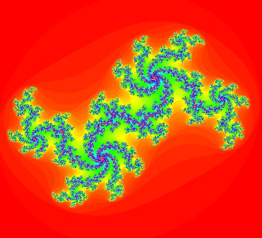
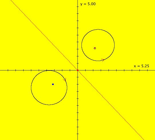
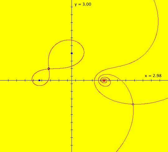
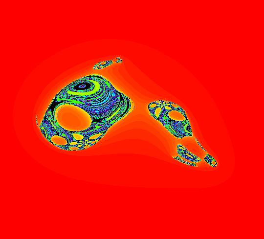
View/Sys/Gal: EMap "AGF: 2 complex lines, EMap" in "AGFEMapExsB."
Range: (vMax,vMin) = (1.551,-3.449), (hMin,hMax) = (-2.085,2.915)
VFld: AGF
This AGF is generated by the lines:
I[1]: (x-1)+i*y = 0, λ₁ = i
I[2]: (x+1)+i*y = 0, λ₂ = (1-i)
The degree of the RHS of the system is: 3.
The trad form of the system is:
dx/dt = (1-x^2+x^3+y^2+x*(-1+4*y+y^2))/4,
dy/dt = (x^2*(-2+y)-2*x*y+(2+y)*(1+y^2))/4.
Image 1: Ode view.
Image 2: EMap view.

View/Sys/Gal: EMap "AGF: 2 complex lines, ver 2, EMap" in "AGFEMapExsB."
Range: (vMax,vMin) = (1.431,-4.158), (hMin,hMax) = (-2.851,2.422)
VFld: AGF
This system is the result of adjusting the 8 parameters for I[1] in system:
        AGF: 2 complex lines, EMap
The AGF is generated by the lines:
I[1]: (1.1+0.01*i)*(x-0.9)+(0.12+0.8*i)*(y-0.01) = 0, λ₁ = (0.03+1.2*i)
I[2]: (x+1)+i*y = 0, λ₂ = (1-i)
The degree of the RHS of the system is: 3.
Image 1: Ode view.
Image 2: EMap view.

View/Sys/Gal: EMap "AGF: 2 complex lines, ver 4, EMap" in "AGFEMapExsB."
Range: (vMax,vMin) = (1.760,-1.206), (hMin,hMax) = (-0.193,1.682)
VFld: AGF
This AGF is generated by the lines:
I[1]: (1.1+0.01*i)*(x-1)+(0.01+0.8*i)*y = 0,
         λ₁ = (0.01+1.1*i)
I[2]: (x+1.4)+(-0.01+0.7*i)*y = 0,
         λ₂ = (1-1.1*i)
The degree of the RHS of the system is: 3.
Image 1: Ode R2+ view.
Image 2: EMap view.

View/Sys/Gal: EMap "AGF: 2 complex lines, ver 5, EMapCT1" in "AGFEMapExsB."
Range: (vMax,vMin) = (0.641,-0.641), (hMin,hMax) = (0.407,1.600)
VFld: AGF
This AGF is generated by the lines:
I[1]: (x-1)+i*y = 0, λ₁ = (0.005+i)
I[2]: (x+1)+i*y = 0, λ₂ = (1-i)
The degree of the RHS of the system is: 3.
Image 1: EMap view.

View/Sys/Gal: EMap "AGF: 2 complex lines, ver 6, EMap" in "AGFEMapExsB."
Range: (vMax,vMin) = (2.500,-2.500), (hMin,hMax) = (-2.500,2.500)
VFld: AGF
This AGF is generated by the lines:
        I[1]: 1.4*(x-1)+1.2*i*y = 0,
         λ₁ = (1.9-0.07*i)
        I[2]: 1.1*(x+1)+i*y = 0,
         λ₂ = (-1.56+0.99*i)
The degree of the RHS of the system is: 3.
Image 1: Ode view.
Image 2: EMap view.

View/Sys/Gal: EMap "AGF: 2 more complex lines, EMapMaxCT1" in "AGFEMapExsB."
Range: (vMax,vMin) = (0.229,-0.053), (hMin,hMax) = (-0.282,-0.067)
VFld: AGF
This AGF is generated by the lines:
I[1]: x+i*y = 0, λ₁ = i
I[2]: (2.1+0.93*i)*(x-0.12)+(-0.62+2*i)*(y-0.15) = 0, λ₂ = (1-i)
The degree of the RHS of the system is: 3.
Image 1: Ode R2+ view.
Image 2: EMap view.

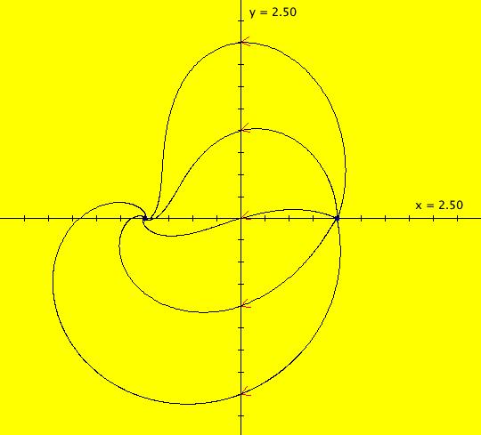
View/Sys/Gal: Ode "AGF: 3 complex lines" in "AGFEMapExsB."
Range: (vMax,vMin) = (3.000,-2.000), (hMin,hMax) = (-2.500,2.500)
VFld: AGF
This AGF is generated by the lines:
        I[1]: x+i*(y-1) = 0, λ₁ = i
        I[2]: (x-1)+i*y = 0, λ₂ = i
        I[3]: (x+1)+i*y = 0, λ₃ = i
The degree of the RHS of the system is: 5.
This is an interesting Ode but it is not a very interesting IMap or EMap.
The generators are three centers and there are two spontaneous saddle points at:
        (x,y) = (+-0.660036,0.242718).
Image 1: Ode view.

View/Sys/Gal: Ode "AGF: 3 complex lines, 1 real line" in "AGFEMapExsB."
Range: (vMax,vMin) = (2.500,-2.500), (hMin,hMax) = (-2.500,2.500)
VFld: AGF
This AGF is generated by the lines:
        L[1]: x-y = 0, m = 1, λ₁ = 0.01
        I[1]: x+i*(y-1) = 0, λ₁ = (-0.1+i)
        I[2]: (x-1)+i*y = 0, λ₂ = (-0.1+i)
        I[3]: (x+1)+i*y = 0, λ₃ = (0.1+i)
The degree of the RHS of the system is: 6.
Image 1: Ode R2+ view.
Image 2: Ode R2 view.

View/Sys/Gal: Ode "AGF: 3 complex lines, 1 real line, ver 2" in "AGFEMapExsB."
Range: (vMax,vMin) = (2.930,-2.070), (hMin,hMax) = (-2.210,2.790)
VFld: AGF
This AGF is generated by the lines:
        L[1]: x-y = 0, m = 1, λ₁ = -0.01
        I[1]: x+i*(y-1) = 0, λ₁ = (-0.1+i)
        I[2]: (1-0.3*i)*(x+0.3)+
                        i*(y-0.82) = 0,
                 λ₂ = (-0.1-1.1*i)
        I[3]: (x+1)+i*y = 0, λ₃ = (0.1+i)
The degree of the RHS of the system is: 6.
An interesting Ode and EMap.
Image 1: EMap CT 1 view.
Image 2: Ode view wo/trajectories.
Image 3: Ode view w/trajectories.

View/Sys/Gal: EMap "AGF: 3 complex lines, ver 2, EMap" in "AGFEMapExsB."
Range: (vMax,vMin) = (3.000,-2.689), (hMin,hMax) = (-2.220,2.976)
VFld: AGF
This AGF is generated by the lines:
        I[1]: x+i*(y-1) = 0, λ₁ = i
        I[2]: (-2+0.5*i)*(x-1)+

                (0.3+2.01*i)*y = 0,
         λ₂ = (-0.15+1.4*i)
        I[3]: (x+1)+i*y = 0, λ₃ = i
The degree of the RHS of the system is: 5.
Image 1: Ode view.
Image 2: EMap view.

View/Sys/Gal: EMap "AGF: 3 complex lines, ver 3, EMap" in "AGFEMapExsB."
Range: (vMax,vMin) = (2.418,-1.616), (hMin,hMax) = (-1.584,1.847)
VFld: AGF
This AGF is generated by the lines:
        I[1]: (1.0001+1.2*i)*(x-0.001)+
                (0.5001+2*i)*(y-1.0001) = 0,
         λ₁ = (-2.06-0.45*i)
        I[2]: (x-1)+i*y = 0, λ₂ = i
        I[3]: (x+1)+i*y = 0, λ₃ = i
The degree of the RHS of the system is: 5.
Image 1: Ode view.
Image 2: EMap view.

View/Sys/Gal: EMap "AGF: 3 complex lines, ver 4, EMap" in "AGFEMapExsB."
Range: (vMax,vMin) = (1.820,-1.780), (hMin,hMax) = (-1.584,2.116)
VFld: AGF
This AGF is generated by the lines:
        I[1]: x+i*(y-1) = 0, λ₁ = i
        I[2]: (1-0.01*i)*(x-1)+
                (-0.04+i)*(y-0.03) = 0,
         λ₂ = (-0.51-1.4*i)
        I[3]: (x+1)+i*y = 0, λ₃ = i
The degree of the RHS of the system is: 5.
Image 1: Ode R2+ view.
Image 2: EMap view.

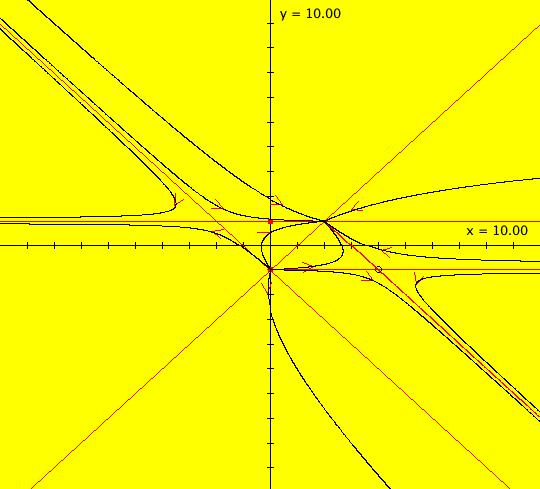
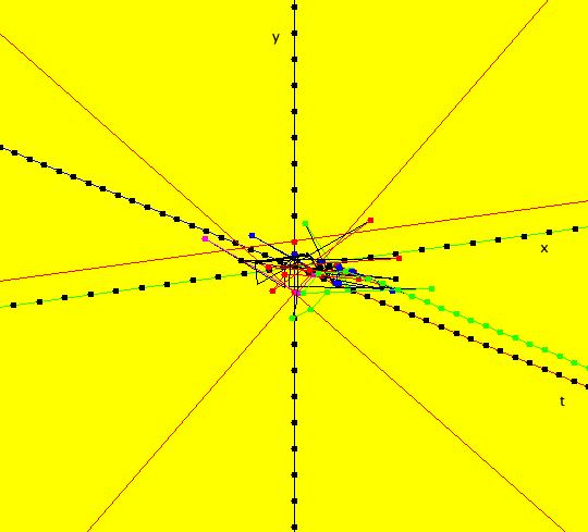
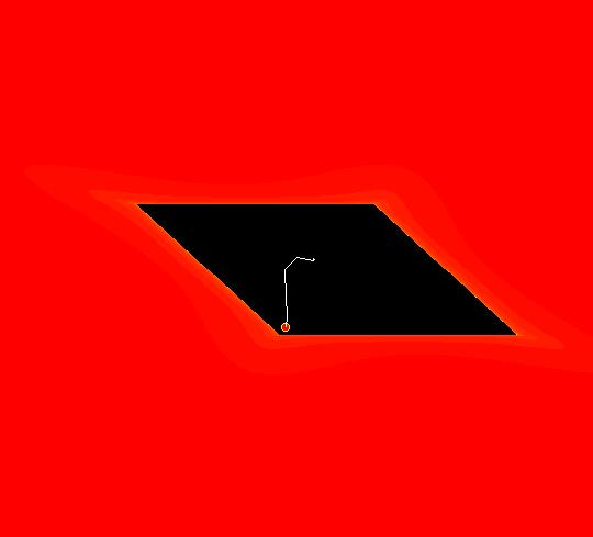
View/Sys/Gal: Ode "AGF: 3 real lines" in "AGFEMapExsB."
Range: (vMax,vMin) = (10.000,-10.000), (hMin,hMax) = (-10.000,10.000)
VFld: AGF
This AGF is generated by the lines:
        L[1]: x-(y+1) = 0, m = 1, λ₁ = 1
        L[2]: x+(y+1) = 0, m = -1, λ₂ = 1
        L[3]: (y-1) = 0, m = 0, λ₃ = 1
The degree of the RHS of the system is: 2.
There are 4 ode fixed points.
Image 1: Ode View.
There is only 1 IMap fixed point at about
        (x,y) = (.6,.3).
Image 2: IMap 3D view. The green orbit parallel to the t axis corresponds to the IMap fixed point.
Image 3: EMap view. All IMap orbits that start inside the black parallelogram (called the "prisoner set") go to the IMap fixed point.

View/Sys/Gal: EMap "AGF: 3 real lines, ver 2, EMap" in "AGFEMapExsB."
Range: (vMax,vMin) = (1.355,-0.542), (hMin,hMax) = (-0.432,1.107)
VFld: AGF
This AGF is generated by the lines:
L[1]: x-0.2381*(y+1) = 0, m = 4.2, λ₁ = 1.2
L[2]: x+(y+1) = 0, m = -1, λ₂ = -5
L[3]: (y-1) = 0, m = 0, λ₃ = -1
The degree of the RHS of the system is: 2.
Image 1: Ode R2+ view.
Image 2: EMap view.
Another fractal.

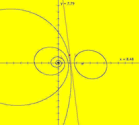
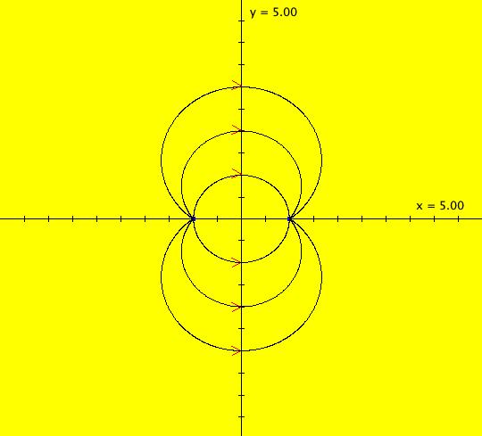
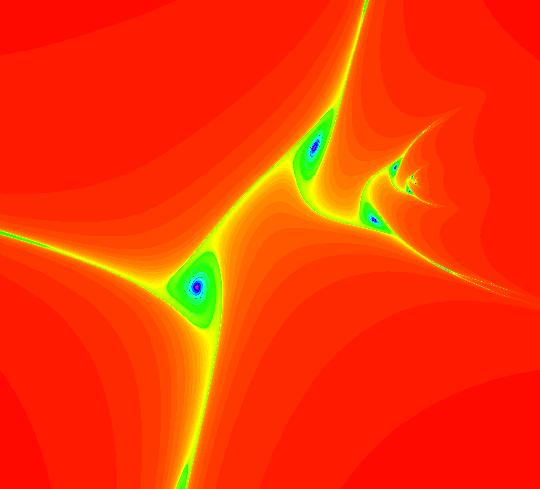
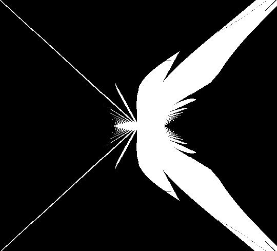
View/Sys/Gal: EMap "AGF: star-out & star-in EMapCT5" in "AGFEMapExsB."
Range: (vMax,vMin) = (5.000,-5.000), (hMin,hMax) = (-5.000,5.000)
VFld: AGF
This AGF is generated by the lines:
I[1]: (x+1)+i*y = 0, λ₁ = 1, star out
I[2]: (x-1)+i*y = 0, λ₂ = -1, star in
The degree of the RHS of the system is: 3.
In traditional (trad) form the system is:
        dx/dt = (y^2-x^2+1)/2,
        dy/dt = -x*y.
When you set p = -1, q = 0, and time-scale by -2, you get:
        dx/dt = x^2-y^2+p,
        dy/dt = 2*x*y+q,
which, as an IMap with c = p+i*q, is the Mandelbrot iteration:
        z <- z^2+c.
The "continuous" Ode views of the this AGF system and the time-scaled version of the system are essentially the same but the discrete-time IMap and EMap views are not.
Image 1: Ode view.
Image 2: EMap view.

View/Sys/Gal: EMap "AGF: trad form of star-out & star-in t-scaled EMapCT5" in "AGFEMapExsB."
Range: (vMax,vMin) = (2.500,-2.500), (hMin,hMax) = (-2.500,2.500)
VFld: (s*(y^2-x^2+1)/2,s*(-x*y)), s = -2.0000;
This iteration is defined by:
        x <- s*(y^2-x^2+1)/2,
        y <- s*(-x*y).
Parameters are:
        s = -2.0000;
EMap CT: 5
This is a time-scaled version of the trad form of the AGF: star-out & star-in. The Ode view trajectories do not change as s changes but the IMap orbits do.
Image 1: Ode view.
Image 2: EMap view.

View/Sys/Gal: EMap "AGF: trad form variation 1 of star-out & star-in, EMap" in "AGFEMapExsB."
Range: (vMax,vMin) = (5.400,-5.700), (hMin,hMax) = (-10.000,10.000)
VFld: (b*x^2-y^2+p,a*x*y%c+q), p = -.70; q = 1.00; a = 1.00; b = .30; c = 6.70;
This system of odes is defined by the equations:
        dx/dt = b*x^2-y^2+p,
        dy/dt = a*x*y%c+q
Parameters are:
        p = -.70; q = 1.00; a = 1.00;
        b = .30; c = 6.70;
The Java mod operator "%" is being used here.
Image 1: Ode view.
Image 2: EMap view.

View/Sys/Gal: EMap "AGF: trad form variation 2 of star-out & star-in, EMap" in "AGFEMapExsB."
Range: (vMax,vMin) = (1.250,-1.250), (hMin,hMax) = (-1.250,1.250)
VFld: (x^2-y^2+p,2*x%y+q), p = -.65; q = 1.00;
This system of odes is defined by the equations:
        dx/dt = x^2-y^2+p,
        dy/dt = 2*x%y+q
Parameters are:
        p = -.65; q = 1.00;
Image 1: Ode view.
Image 2: EMap view.

View/Sys/Gal: EMap "AGF: trad form variation 3 of star-out & star-in, EMapMaxCT9" in "AGFEMapExsB."
Range: (vMax,vMin) = (5.000,-5.000), (hMin,hMax) = (-5.000,5.000)
VFld: (x^2-y^2+p,2*x%y+q), p = .7000; q = -6.9000;
This iteration is defined by:
        x <- x^2-y^2+p,
        y <- 2*x%y+q.
Parameters are:
        p = .7000; q = -6.9000;
EMap CT: 9
Image 1: Ode view.
Image 2: EMap view.