Click on an image to go directly to a system or scroll to see all of the systems in this gallery.
 |
 |
 |
 |
 |
 |
 |
 |
 |
 |
 |
 |
 |
 |
 |
 |
 |
 |
 |
 |
 |
 |
 |
 |
 |
 |
 |
 |
 |
 |
 |
 |
 |
 |
 |
 |
 |
 |
 |
 |
 |
 |
 |
 |
 |
 |
 |
 |
 |
 |
 |
 |
 |
 |
 |
 |
 |
 |
 |
 |
 |
 |
 |
 |
 |
 |
 |
 |
 |
 |
 |
 |
 |
 |
 |
 |
 |
 |
 |
| OdeFactory Images and Annotations | |||||||||||||||||||||||||||||||||||||||||||||||||||||||||||||||||||||||||||||||||||||||||||||||||||||||||||||||
|
|
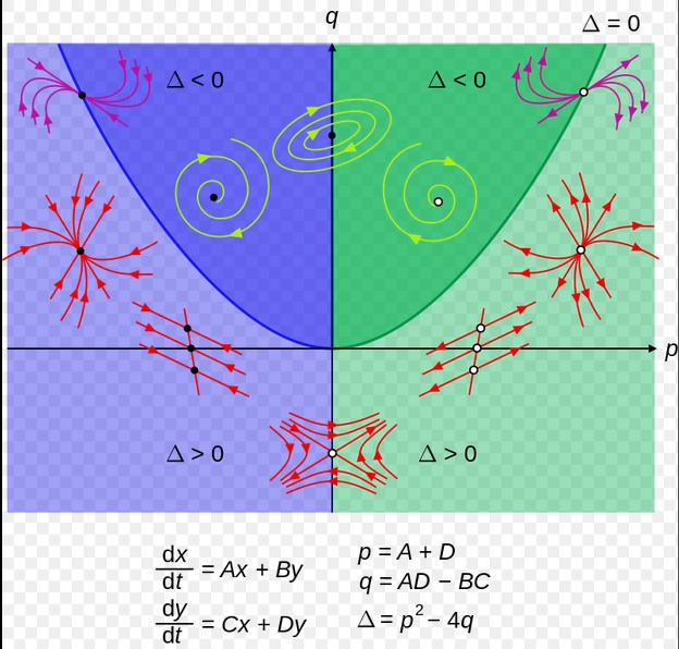
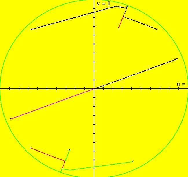
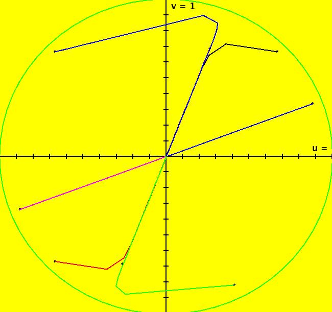
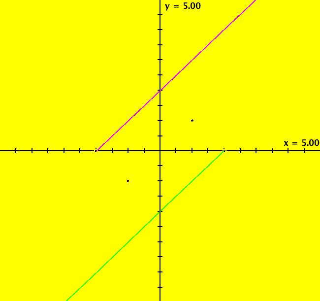
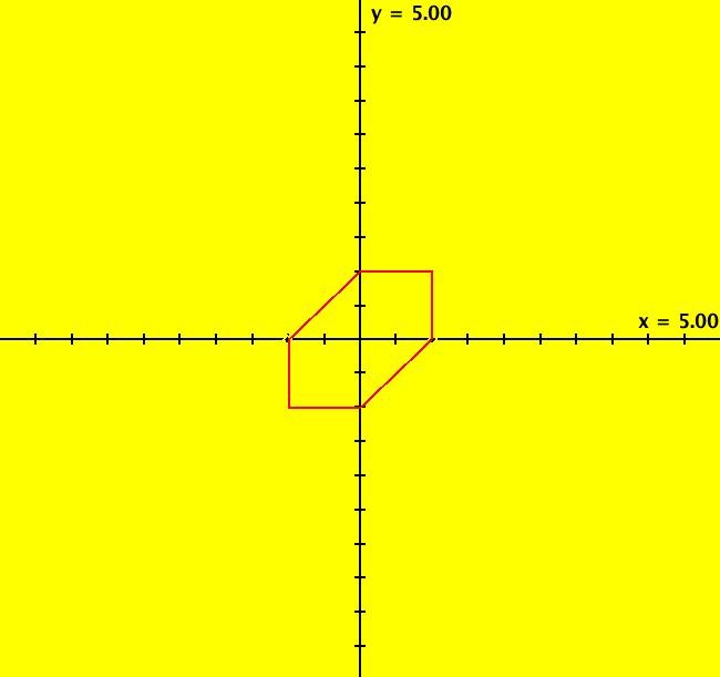
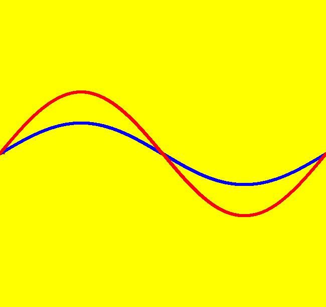
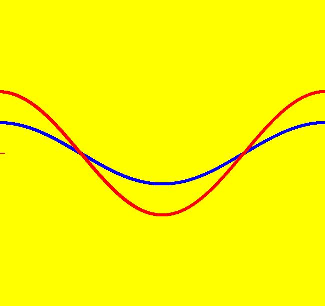
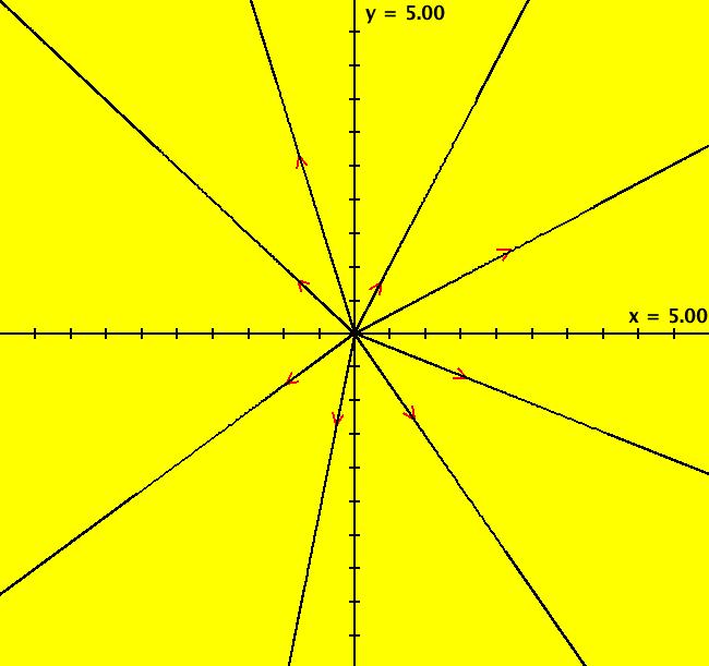
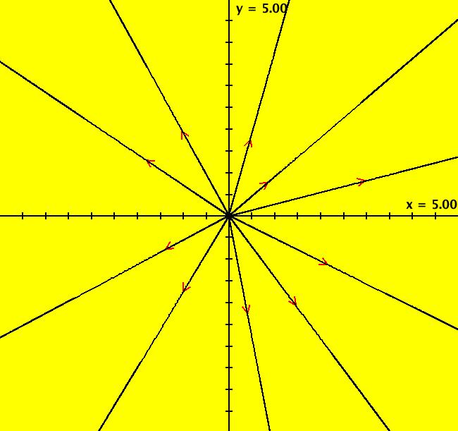
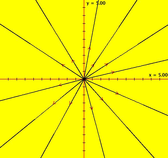
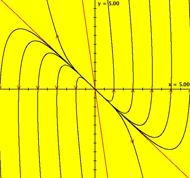
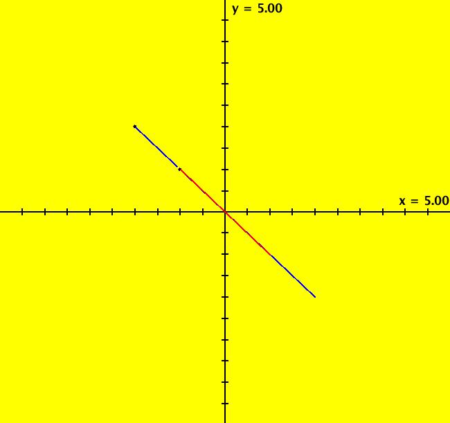
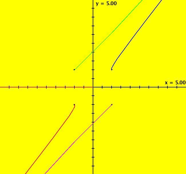
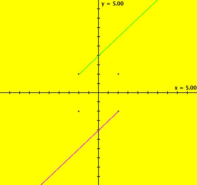
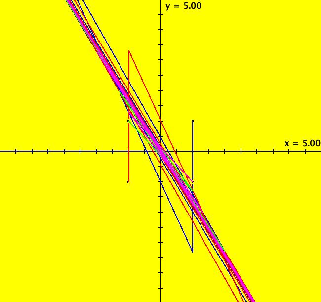
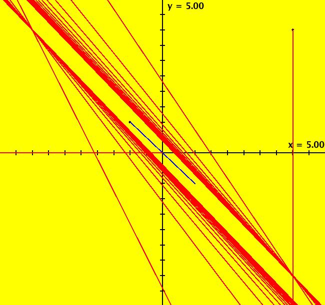
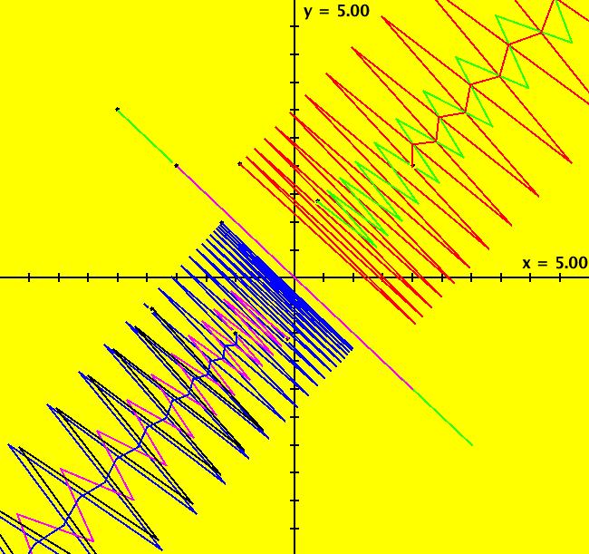
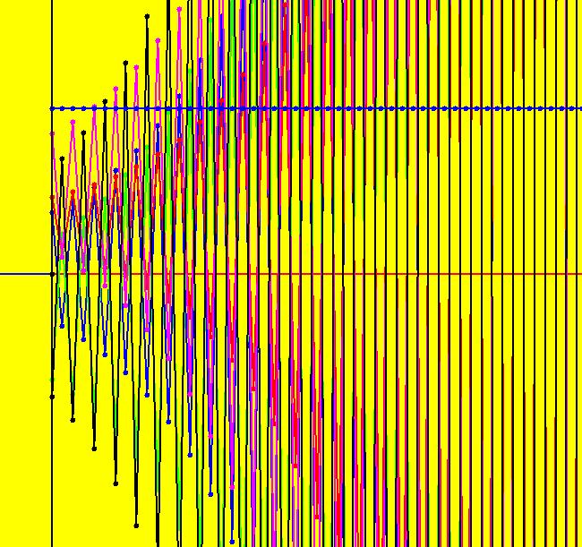
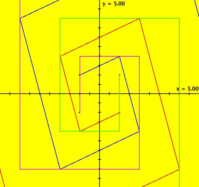
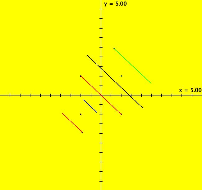
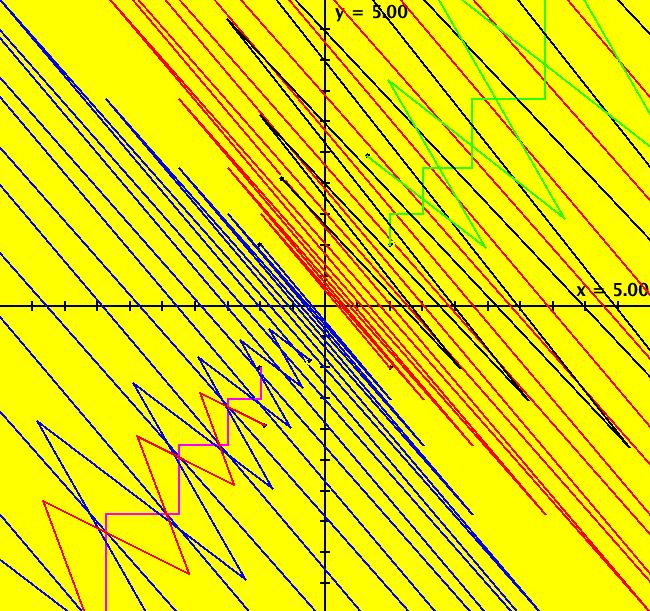
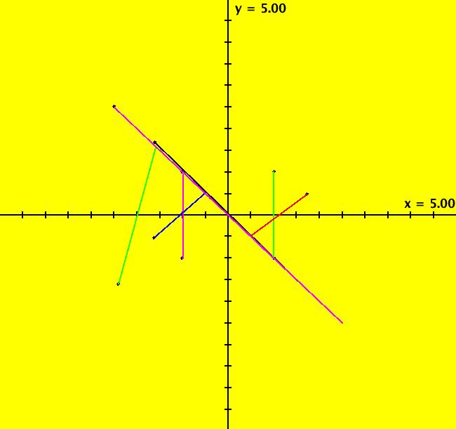
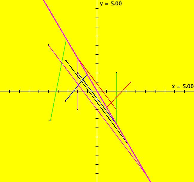
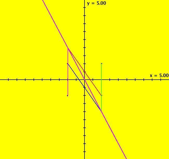
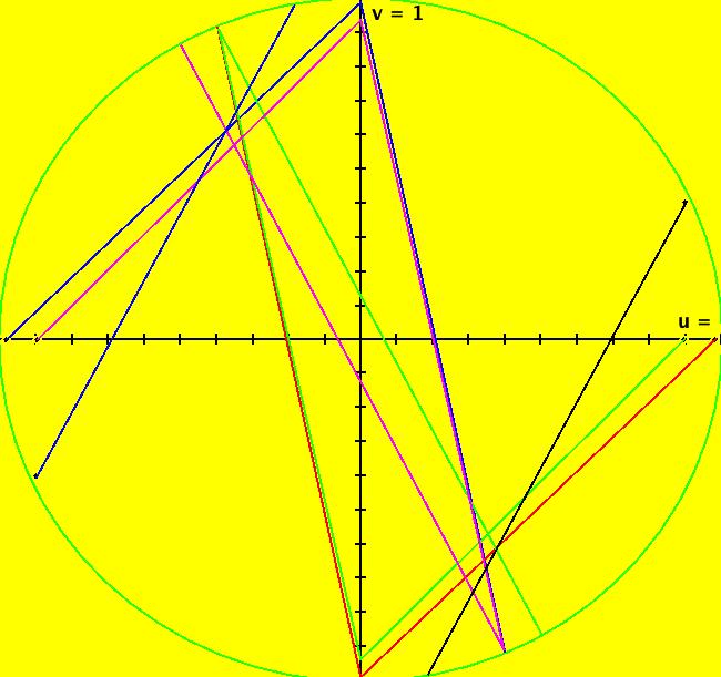
View/Sys/Gal: Ode " Overview" in "2DLinearVectorFields." ---- Classifing 2D Linear Systems The purpose of this gallery is to demonstrate how to use OdeFactory to find out all there is to know about Odes or IMaps defined by 2D linear vector fields. We first reduce the dimension of the parameter space (i.e. the number of parameters needed to define all of the 2D linear vector fields) from four to two. Then we identify all of the topologically different kinds of trajectories for Odes and orbits for IMaps. ---- Definition of a 2D Linear Vector Field A 2D linear vector linear field is defined by: (Vx,Vy) = (a*x+b*y,c*x+d*y), or in WA matrix notation, by {Vx,Vy} = {{a,b},{c,d}}*{x,y}. From the point of view of linear algebra the vector field defines a static linear transformation of R2 into R2. The static vector field can be viewed in OdeFactory by using the "V On/Off" button. ---- Flows in a Vector Field When a time sequence of transformations is considered the vector field defines a dynamic transformation of the plane. The "Flow" button can be used to show the motion of the flow in the vector field. ---- Views: Ode, IMap, EMap Dynamic transformations can be: (a) continuous: Ode view, RK4 iteration algorithm with "time" step ≃ .01 or (b) discrete: IMap view, simple iteration with "time" step = 1. The EMap view is a variation of an IMap view that uses the escape-time algorithm. ---- 3D View, the R2+ View The 3D view shows the (x,y) phase plane and the perpendicular t axis. The R2+ view, which is the Poincare compactification of R2 onto the unit disk, shows the global phase portrait of a system. ---- Classification Of 2D Linear Odes The phase space portraits of 2D linear systems, both in the Ode view and the IMap view, can be classified using the discriminate of the characteristic polynomial (see Consider the system: dx/dt = a*x+b*y, dy/dt = c*x+d*y or, in matrix form, dX/dt = A*X. The origin is always a fixed point in the Ode view. Let p be the trace of A and q the determinant of A: p = a+d, q = a*d-c*b. The characteristic polynomial of the system is: λ^2-p* λ+q = 0. The eigenvalues and eigenvectors of the system are: λ1 = (p-sqrt(disc))/2, v1 = ( λ2,1) λ2 = (p+sqrt(disc))/2, v2 = ( λ1,1) where disc = p^2-4*q is the discriminate of the system. Note that p = λ1+ λ2, q = λ1* λ2 so m1 = slope of v1 = λ1/q and m2 = slope of v2 = λ2/q. The bifurcation space of the system is the minimum parameter space, which in this case is the (p,q) plane. The parabola q = p^2/2 partitions the bifurcation space into the regions inside and outside of the parabola. The parabola, the positive q axis and the p axis are the bifurcation curves. Image 1: The Ode bifurcation diagram in the (p,q) plane. (A) Inside the parabola the eigenvalues are complex and the corresponding trajectories in the phase space are spirals and centers. We get spirals if p ≠ 0 and centers if p = 0. The periods of the centers are a function of q. They range from ∞ for q = 0 to 0 for q = ∞. (B) Outside the parabola, for q > 0, the trajectories are nodes. (C) On the parabola the trajectories are stars and degenerate nodes. We get stars when the coefficient matrix is a multiple of the identity matrix and degenerate nodes when λ1 = λ2 = real and v1 = v2. (D) On the p axis the trajectories are straight lines and y = 0 consists of fixed points. (E) For q < 0 the trajectories are saddle nodes, i.e. hyperbolas. The eigenvalues are real. ---- Classification of 2D Linear IMaps The question is: when viewed as an IMap, is the same classification scheme possible for the orbits of the corresponding iteration map? The answer is: sort of but not exactly. First note that a time-scaling parameter s does not change the classification scheme in the Ode case but it does add an additional bifurcation parameter for IMaps. Image 2: The IMap bifurcation diagram in the (p,q) plane. Note - in the diagram read the "x" axis as p and the "y" axis as q. For 2D linear IMap orbits we get spirals and cycles inside the q = p^2/4 parabola. On the q = 1 line, with p ∈ [-2,2), we get cycles. Above q = 1 we get cw spirals out and below q = 1 we get cw spirals in. See systems (10) through (16) for the details. ---- Analytic Solutions There are analytic solutions for linear Ode systems but not for linear IMap systems. The fundamental theorem for linear ode systems says that the analytic solution to the system dX/dt = A*X is X(t) = e^(A*t)*X(0). Apply WA to {x,y}=MatrixExp[{{a,b},{c,d}}t].{x0,y0} to view the analytic solution. ---- AGFs AGFs are Algebraically Generated Flows. A flow defined by the 2D vector field (Vx,Vy) = (a*x+b*y,c*x+d*y) can also be written as AGF by using the eigenvalues and eigenvectors of the coefficient matrix of a 2D linear system to create the AGF. The advantage of the AGF form is that it enables you to dynamically change the defining geometric properties of the vector field by using the field's eigenvalue and eigenvector controllers. AGFs extend to 2D nonlinear polynomial systems where the generators consist of real and complex lines. ---- The Simplified General Form This is a simplified 2-parameter version of the 4-parameter linear system where the two parameters are the trace p and the determinant q: dx/dt = y, dy/dt = -q*x+p*y. In matrix form, the system is: dX/dt = A*X, where A = {{0, 1},{-q,p}}. There are eight topologically distinct types of Ode phase space images. The last system is: B = I = {{1,0},{0,1}}.
(p,q) (3,1) (2,1) (1,1) (0,1) (p,0) (0,0) (p,-1) B = I
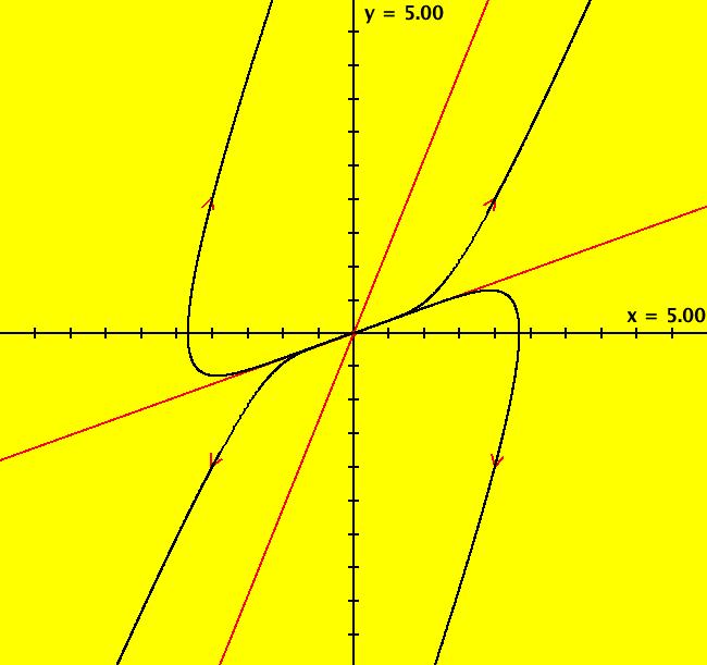
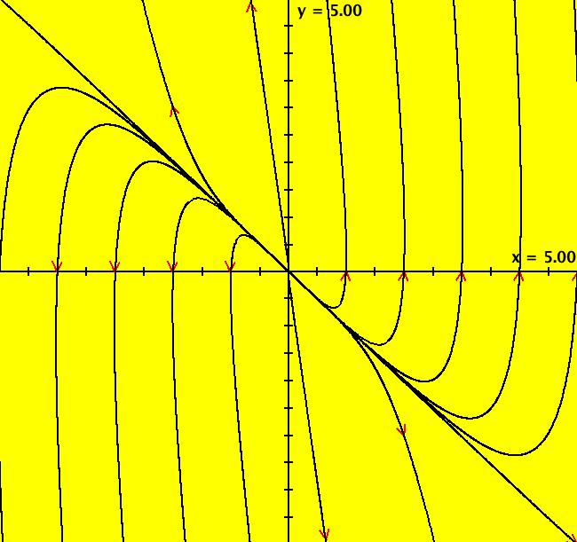
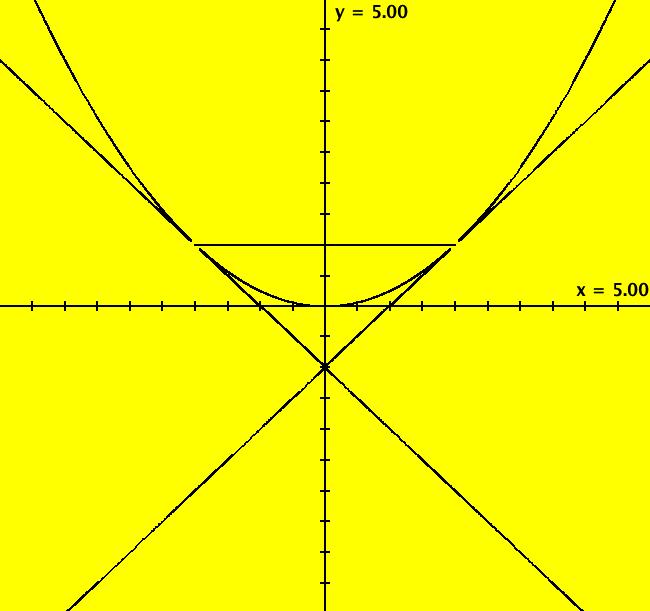
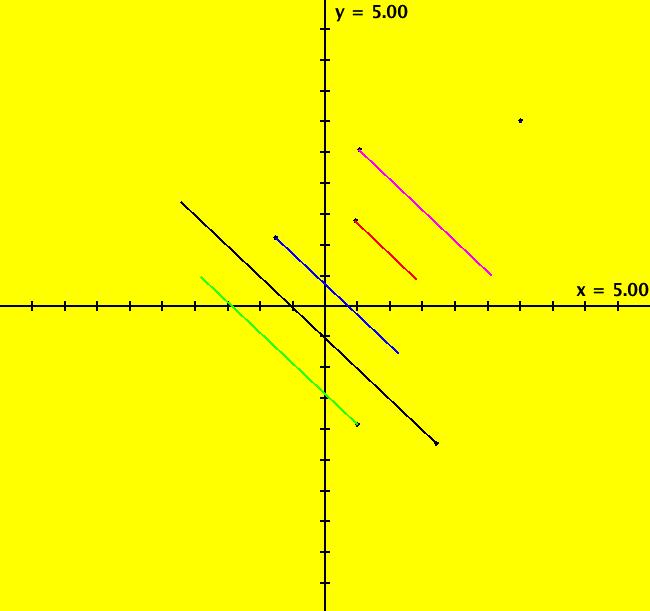
Note that only nondegenerate nodes and spirals are stable in the parameter space. If λ is real, the motion on L is out iff λ > 0. If λ is complex, the motion in (r, θ) is dr/dt > 0 (out) iff re( λ) > 0 and d θ/dt > 0 (ccw) iff im( λ) < 0. Image 3: An Ode saddle node.
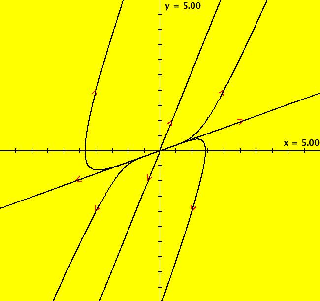
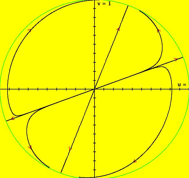
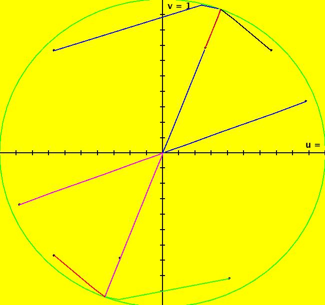
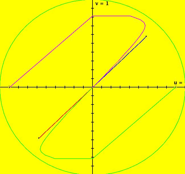
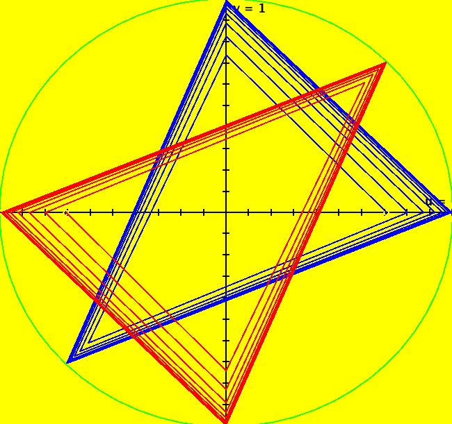
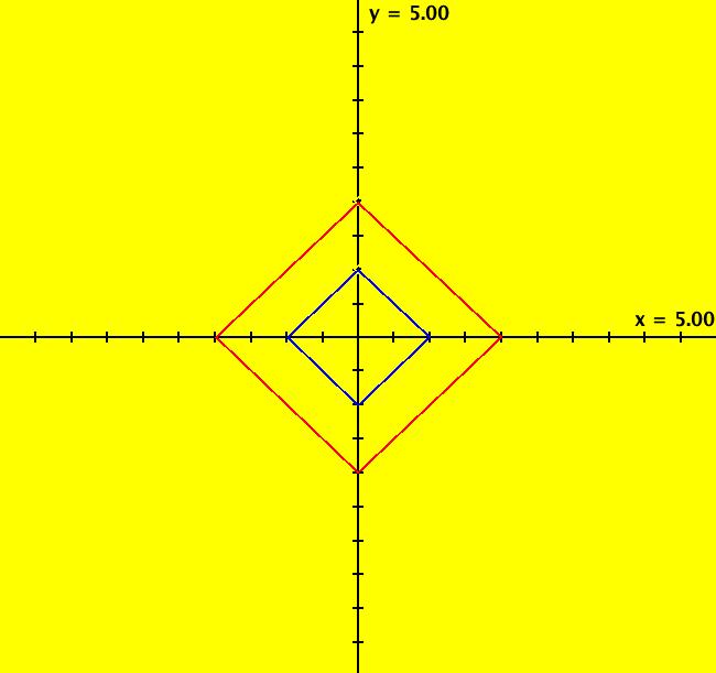
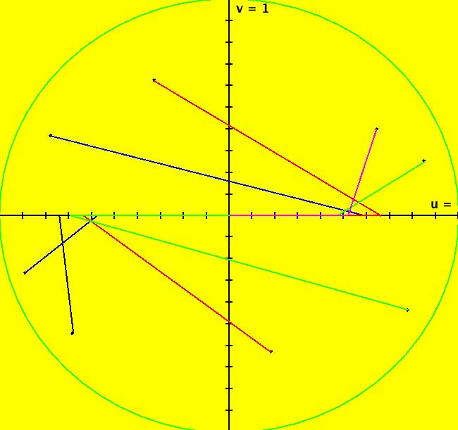
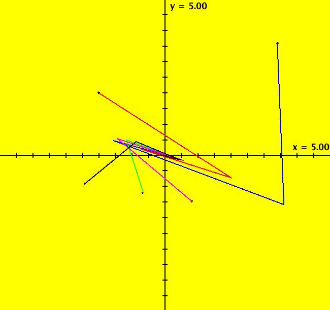
View/Sys/Gal: Ode "( 1) (p,q) = (3,1) node" in "2DLinearVectorFields." This system of odes is defined by the equations: dx/dt = s*y, dy/dt = s*(-q*x+p*y). Parameters are: q = 1.0000; p = 3.0000; s = 1.0000; A = {{0,1},{-1,3}} λ1 = (3+sqrt(5))/2, v1 = (1/ λ1,1), m1 = λ1/q = λ1 λ2 = (3-sqrt(5))/2, v1 = (1/ λ2,1), m2 = λ2/q = λ2 and since q = 1 λ1 = m1 = 2.61803 λ2 = m2 = .381966 Since the flow is out from the fixed point at (0,0), this is called an unstable node. Setting s = -2 converts it to a stable node. Image 1: Ode view, unstable node. The straight lines form the separatrix system for the system. See the R2+ view. Image 2: Ode R2+ view. In the IMap view, there are IMap/EMap bifurcation points near s = +-.3 where the maps flip between unstable and stable. Image 3: IMap R2+ view, s = 1 Image 4: IMap R2+ view, s = .4 Image 5: IMap R2+ view, s = .3
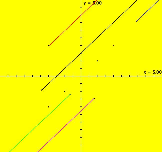
View/Sys/Gal: Ode "( 1) node, AGF" in "2DLinearVectorFields." NOTE: All of the different kinds of linear 2D Ode systems can be defined using real and complex linear generators. The parameters in the generators are related to the eigenvectors and eigenvalues of the 2 by 2 coefficient matrix A where dX/dt = A*X. Such systems are called "AGF" systems (Algebraically Generated Flows). Nonlinear AGF Ode systems can be defined by specifying local behavior at fixed points. This AGF is generated by the lines: L[1]: x-0.381967*y = 0, m1 = 2.61803, λ1 = 2.61803 L[2]: x-2.618034*y = 0, m2 = 0.381966, λ2 = 0.381966 The degree of the RHS of the system is: 1. Note that for a pair of linear generators centered at (0,0): mi = λi = 1/ λj The generators, L[1] and L[2], shown in red, are the separatrices. Image 1: Ode view. Here is the system in the traditional form: dx/dt = (-1.253*(0.357*x-0.934*y)+ 0.479*(0.934*x-0.357*y)), dy/dt = -((3.281*(0.357*x-0.934*y)- 0.183*(0.934*x-0.357*y))), which simplifies, via WA, to: dx/dt = y, dy/dt = -x+3*y, which is system "( 1) (p,q) = (3,1) node."
View/Sys/Gal: EMap "( 2) (p,q) = (2,1) degenerate node" in "2DLinearVectorFields." This system of odes is defined by the equations: dx/dt = s*y, dy/dt = s*(-q*x+p*y). Parameters are: q = 1.00; p = 2; s = 1 Here (p,q) is a point on the top half of the parabola. Image 1: Ode view, degenerate unstable node. Select "Show 2D IMap Orbit Sequence" on the Help menu then go to the IMap view. In the IMap view, for s = 1, seeds on the y = x line are fixed points since x <- y = x, y <- -x+2*y = -y+2*y = y and all other seeds give straight line orbits with slope 1 since Δy/ Δx = (-x+2*y-y)/(y-x) = 1. Image 2: IMap view, s = 1. Investigate the IMap in the range -1 < s < 1 in the R2+ view. Image 3: IMap view in R2+ with s = .7. See the EMap view near |s| = 1. Image 4: EMap view with s = 1.
View/Sys/Gal: Ode "( 2) degenerate node, AGF" in "2DLinearVectorFields." This AGF is generated by the lines: L[1]: x-y = 0, m1 = 1, λ1 = 1 L[2]: x-1.010101*y = 0, m2 = 0.99, λ2 = 0.99 The degree of the RHS of the system is: 1. This is a limit flow. L[2] -> L[1]. Image 1: Ode R2+ view.
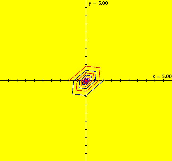
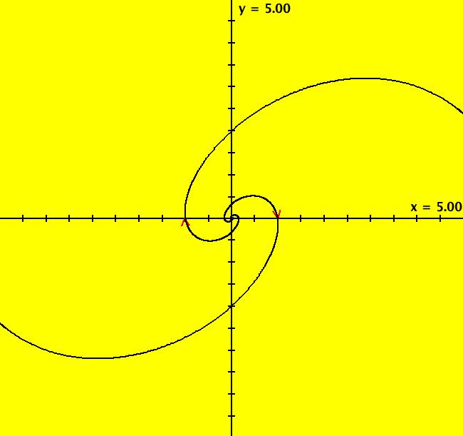
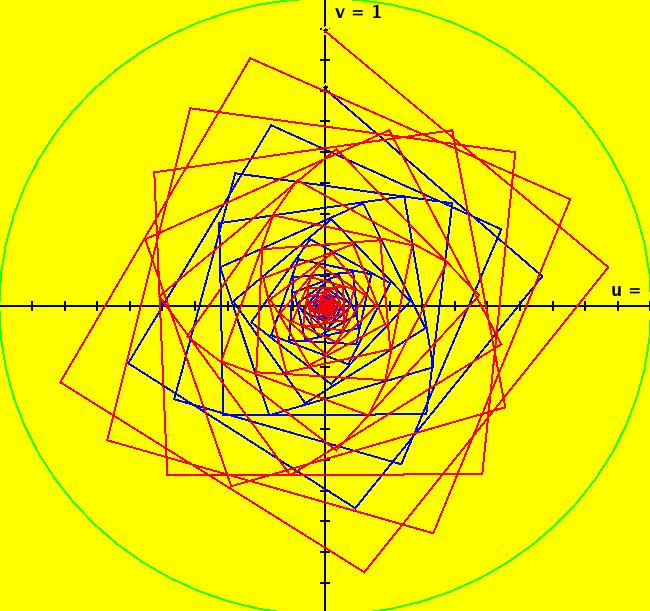
View/Sys/Gal: Ode "( 3) (p,q) = (1,1) spiral" in "2DLinearVectorFields." This system of odes is defined by the equations: dx/dt = s*y, dy/dt = s*(-q*x+p*y). Parameters are: q = 1.00; p = 1; s = 1 Here (q,p) is a point inside the parabola but above the q axis. In the Ode view, we get: spirals out for s > 0 and spirals in for s < 0. Image 1: Ode R2+ view, spirals out. In the IMap view, we get:
Image 2: Image 3: Image 4: Image 5: Image 6:
Image 7: IMap R2+ view with s = -1.1 several spirals out. There is a somewhat interesting EMap for s = 1.1. Image 8: EMap CT 1 view with s = 1.1.
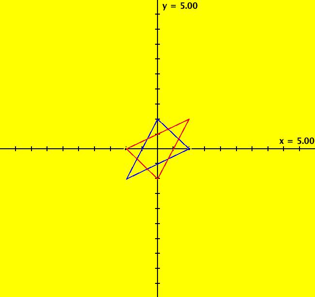
View/Sys/Gal: Ode "( 3) spiral, AGF" in "2DLinearVectorFields." This AGF is generated by the lines: I[1]: 1.1*x+(-0.42+i)*y = 0, λ1 = (0.5+0.866025*i) The degree of the RHS of the system is: 1. Image 1: Ode view cw spiral out. Image 2: IMap view, hexagons.
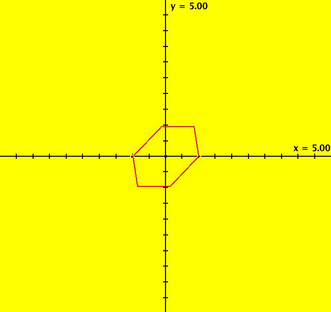
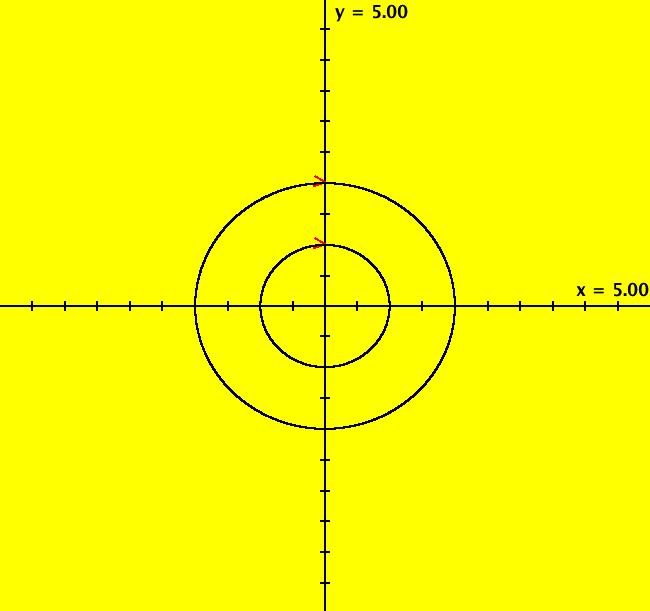
View/Sys/Gal: Ode "( 4) (p,q) = (0,1) center" in "2DLinearVectorFields." This system of odes is defined by the equations: dx/dt = s*y, dy/dt = s*(-q*x+p*y). Parameters are: q = 1.00; p = .00; s = 1 Here (q,p) is inside the parabola and on the q axis. In the Ode view we get cycles, cw for s > 0. Image 1: Ode view, cycles with period = 2 π. In the IMap view we get squares for |s| = 1 (4-cycles) and spirals for |s| ≠ 1. The spirals are out for |s| > 1. The motion is cw for s > 0. Image 2: IMap view, s = 1, squares with period 4. Image 3: IMap view in R2+, p = .15, q = 1.1, s = .9 Start several seeds with s = 1.1 in the R2+ IMap view, with the orbit sequence lines on, and the axes and seeds off. Also set (q,p) = (1.1,.07) then adjust s.
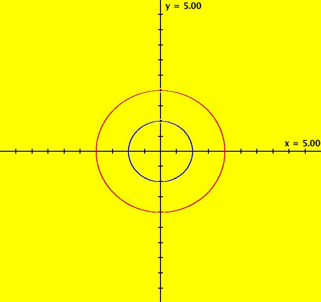
View/Sys/Gal: Ode "( 4) center, AGF" in "2DLinearVectorFields." This AGF is generated by the lines: I[1]: x+i*y = 0, λ1 = i The degree of the RHS of the system is: 1. In trad form: dx/dt = y, dy/dt = -x. Image 1: Ode view, cycles with period = 2 π.
View/Sys/Gal: Ode "( 4) center, H=(x^2+y^2)/2" in "2DLinearVectorFields." This system of odes is defined by the equations: dx/dt = (a*((4*y)/4)), dy/dt = -(a*((4*x)/4)). Parameters are: a = 1; Functions are: H=(x^2+y^2)/2 The system is a time-scaled version of: dx/dt = y, dy/dt = -x. Note that H factors into the product of the complex line I[1] = x+i*y and its complex conjugate: H = (x+i*y)*(x-i*y)/4. Image 1: Ode view, cycles with period = 2 π.
View/Sys/Gal: IMap "( 4b) (p,q) = (0,1) center IMap, Euler's ode method" in "2DLinearVectorFields." System ( 4), in the Ode view, was defined by the equations: dx/dt = s*y, dy/dt = s*(-q*x+p*y), with parameters, q = 1.00; p = .00; s = 1. The RK4 method gave circles. If you consider the approximate system as: Δx = xNew -xOld ~ Δt*y, Δy = yNew -yOld ~ Δt*(-q*x+p*y) with Δt = s = .001 then you get the iteration: x <- s*y+x, y <- s*(-q*x+p*y)+y. with parameters q = 1.0000; p = .0000; s = .0010; This is Euler's method applied to the ode system. Image 1: IMap view. Image 2: 3D/(t,x) IMap view w/hMax = 2 π/.001 = 6283 Image 3: 3D/(t,y) IMap view w/hMax = 2 π/.001 = 6283
View/Sys/Gal: Ode "( 5) (p,q) = (1,0) fixed points on y = 0" in "2DLinearVectorFields." This system of odes is defined by the equations: dx/dt = s*y, dy/dt = s*(-q*x+p*y). Parameters are: q = .00; p = 1.00; s = 1.00; Keep q = 0, p and s may vary. ----- In the Ode View The x axis consists of fixed points for all p and s. ----- In the IMap View The IMap view is more complicated than the Ode view. We can get: fixed points on y = x, 2-cycles on y = -x or a single fixed point at (0,0). With q = 0, s = 1:
Image 1 2 3 4
View/Sys/Gal: Ode "( 5) fixed points on y = 0, AGF" in "2DLinearVectorFields." This AGF is generated by the lines: L[1]: x-y = 0, (in red) m1 = 1, λ1 = 1 L[2]: y = 0, (in red) m2 = 0, λ2 = 0 The degree of the RHS of the system is: 1. Image 1: Ode view.
View/Sys/Gal: IMap "( 6) (p,q) = (0,0) fixed points on y = 0" in "2DLinearVectorFields." This system of odes is defined by the equations: dx/dt = s*y, dy/dt = s*(-q*x+p*y). Parameters are: q = .00; p = .00; s = 1.00; The system is just: dx/dt = y, dy/dt = 0. Image 1: Ode view. In this case, for s = 1, the IMap seed (x,y) -> (y,0) -> (0,0) in at most two iterations. For example, (2,1) -> (1,0) -> (0,0) and (1,0) -> (0,0). Image 2: 3D/(t,x,y) IMap view. Try other values of s.
View/Sys/Gal: Ode "( 6) fixed points on y = 0, AGF" in "2DLinearVectorFields." This AGF is generated by the lines: L[1]: (y-1) = 0, (in red) m1 = 0, λ1 = 1 L[2]: (y+1) = 0, (in red) m2 = 0, λ2 = -1 The degree of the RHS of the system is: 1. Generally L[1] and L[2] would be separatrices but in this degenerate case they are not. The x axis is the only separatrix. Image 1: Ode R2+ view.
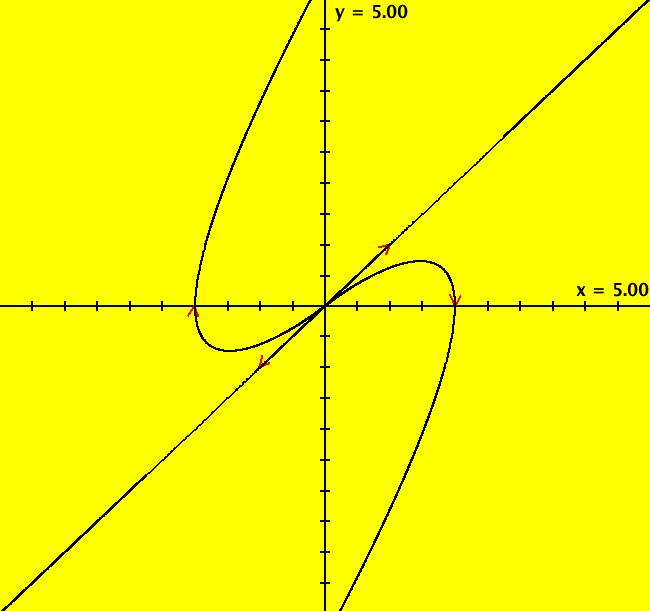
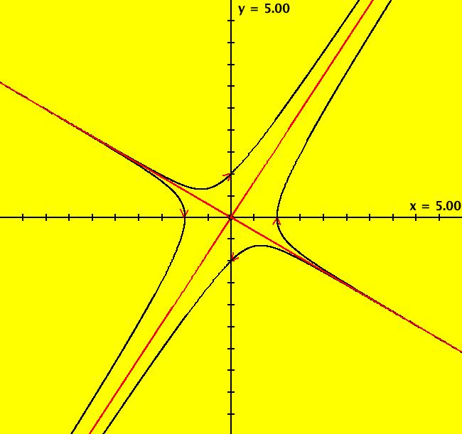
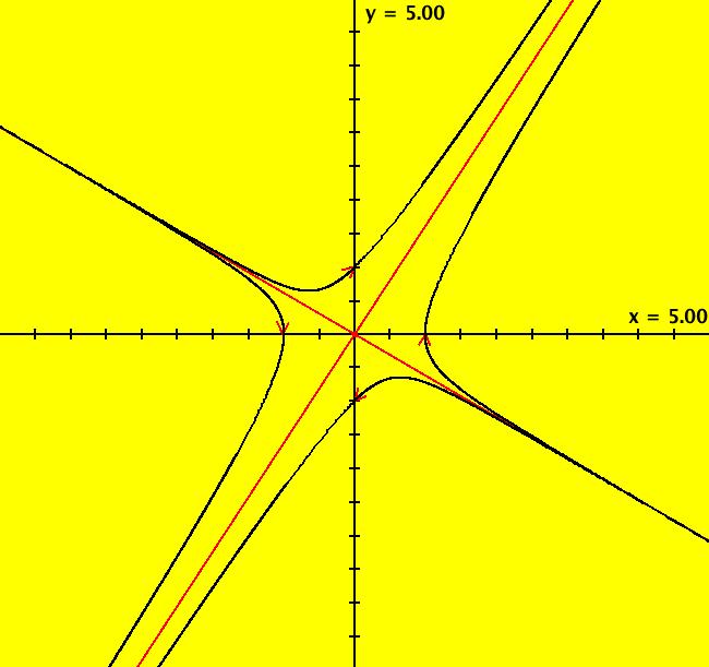
View/Sys/Gal: Ode "( 7) (p,q) = (1,-1) saddle" in "2DLinearVectorFields." This system of odes is defined by the equations: dx/dt = s*y, dy/dt = s*(-q*x+p*y). Parameters are: q = -1.00; p = 1.00; s = 1.00; The red lines, which are approximate separatrices in the Ode view, are in the directions of the eigenvectors. The eigenvalues are real and have different signs. Applying WA to {{0,1},{1,1}} gives λ1 = 1.61803, v1 = (.618034,1), m1 = 1/.618034 = λ1, λ2 = -.618034, v2 = (-1.61803,1), m2 = 1/-1.61803 = λ2. Image 1: Ode view: q = -1, p = s = 1.00. Image 2: IMap view: q = -1, p = 0, s = 1, 2-cycles on y = a-x, fixed points on y = x. For p = 0, s = +-1 are bifurcation values in the IMap and EMap views. Image 3: IMap view for: q = -1, p = 0, s = -1.1 Try varying s in the IMap view in R2+.
View/Sys/Gal: Ode "( 7) saddle, AGF" in "2DLinearVectorFields." This AGF is generated by the lines: L[1]: x-0.618036*y = 0, m1 = 1.61803, λ1 = 1.61803 L[2]: 1*x+1.618034*y = 0, m2 = -0.618034, λ2 = -0.618034 The degree of the RHS of the system is: 1. Image 1: Ode view.
View/Sys/Gal: Ode "( 8) B = I = {{1,0},{0,1}} p=q=1 star" in "2DLinearVectorFields." The coefficient matrix of this system is {{1,0},{0,1}}, which is not of the form {{0, 1},{-q, p}}. The system of odes is defined by the equations: dx/dt = x, dy/dt = y. The eigenvalues are λ1 = λ2 = (2+-sqrt(4-4))/2 = 1 In the IMap view, every point is a fixed point. Image 1: Ode view, star out.
View/Sys/Gal: Ode "( 8) star, AGF, 1 complex line" in "2DLinearVectorFields." This AGF is generated by the lines: I[1]: x+i*y = 0, λ1 = 1 The degree of the RHS of the system is: 1. Since λ1 is real there is no angular motion. In trad form the system is: dx/dt = x, dy/dt = y. The system's name says "1 complex line" but whenever you select a complex line as a generator the complex conjugate of the line is included in the AGF to keep the vector field real. So - from the user's point of view this AGF is generated by 1 complex line. Image 1: Ode view, star out.
View/Sys/Gal: Ode "( 8) star, AGF, 2 real lines" in "2DLinearVectorFields." This AGF is generated by the lines: L[1]: y = 0, (in red) m1 = 0, λ1 = 1 L[2]: x = 0, (in red) m2 = inf, λ2 = 1 The degree of the RHS of the system is: 1. In trad form the system is: dx/dt = x, dy/dt = y. There is no angular motion because λ1 = λ2. Image 1: Ode view, star out.
View/Sys/Gal: Ode "( 9) {{.5,-1.6},{12,14}} in trad form" in "2DLinearVectorFields." The purpose of this example is to show how to get from a more general 2D linear system to the corresponding AGF. This system of odes is defined by the equations: dx/dt = .5*x-1.6*y, dy/dt = 12*x+14*y. The system gives an unstable (out) flow. Image 1: Ode view. The two straight line trajectories are in the eigenvector directions. Since the system is not a center or spiral, the AGF generators are a pair of real lines, L[1] and L[2], through the origin in the directions of the eigenvectors. The flow rates on L[1] and L[2] are the eigenvalues. First apply WA to {{.5,-1.6},{12,14}} to find the eigenvectors and eigenvalues. Using the eigenvectors v1 = (0.133426, -0.991059), v2 = (-0.703677, 0.71052). we can compute the slopes of L[1] and L[2] m1 = v1y/v1x = -7.42566 and m2 = v2y/v2x = -1.0097246 The eigenvalues are λ1 = 12.3844, λ2 = 2.11556 Create the AGF by using mi and λi to define L[i].
View/Sys/Gal: Ode "( 9) {{.5,-1.6},{12,14}}, as AGF" in "2DLinearVectorFields." This AGF is generated by the lines: L[1]: x+0.134668*y = 0, (in red) m1 = -7.42566, λ1 = 12.3844 L[2]: 1*x+0.990369*y = 0, (in red) m2 = -1.009725, λ2 = 2.11556 The degree of the RHS of the system is: 1. Image 1: Ode view. The two generators, L[1] and L[2], are in the eigenvector directions. As a check, the trad form of the AGF is: dx/dt = (-2.743*(0.711*x+0.704*y)+ 2.471*(0.991*x+0.133*y)), dy/dt = -((-20.369*(0.711*x+0.704*y)+ 2.495*(0.991*x+0.133*y))), which simplifies (via WA) to dx/dt = 0.498488*x-1.60243*y, dy/dt = 12.0098*x+14.0079*y, which, within the computation roundoff errors in the eigenvalues and eigenvectors, is correct.
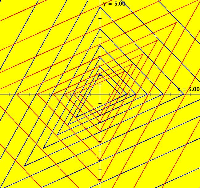
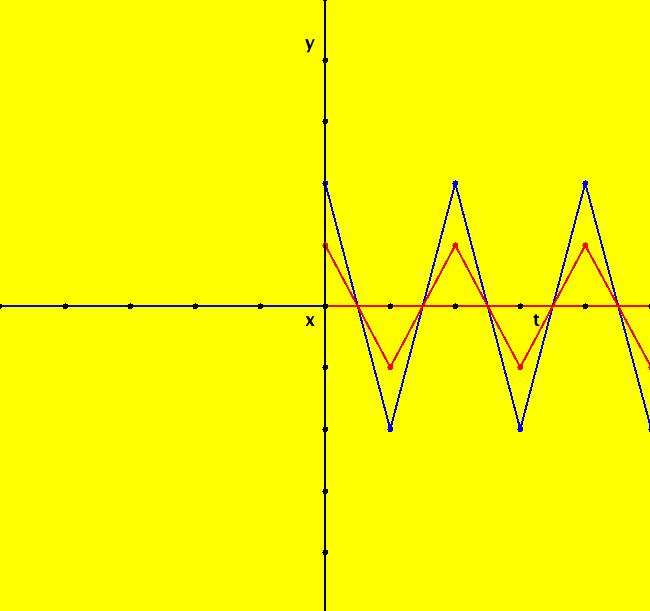
View/Sys/Gal: IMap "(10) Bifurcation Diagram for 2D Linear IMap1100s" in "2DLinearVectorFields." This iteration is defined by: x <- y, y <- -q*x+p*y. Parameters are: p=-2; q=1 The coefficient matrix of the system is: {{0,1},{-q,p}}. Note that p is the trace and q is the determinant of the matrix. For p = -2 and q = 1 we get period-2 orbits for ICs on y = -x and orbits that oscillate between +- ∞ for ICs not on y = -x. Image 1: IMap view, per-2 orbits starting on y = -x. Image 2: IMap 3D/(t,y) view. Systems (11) through (15) are used to show how to find the bifurcation diagram for 2D linear IMaps. The IMap bifurcations occur in the (p,q) IMap bifurcation plane on the lines: q = p^2/4, q = 1, p+q = -1 and p-q = -1. See Discrete Chaos by Saber Elaydi.
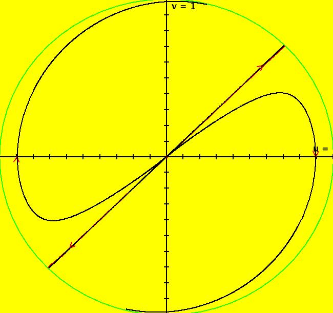
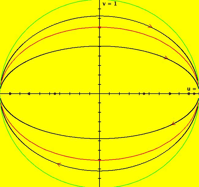
View/Sys/Gal: Ode "(10b) the (p,q) bifurcation plane for (x,y) <- (y,-q*x+p*y)" in "2DLinearVectorFields." This quasiHamiltonian system of odes, defined by the equations: dx/dt = (a*D*A*B+b*C*A*B+c*C*D*B+d*C*D*A), dy/dt = -(a*(-1)*D*A*B+b*C*A*B+ c*(-1*((8*x)/16))*C*D*B), with parameters: a = 1; b = 1; c = 1; d = 1; and functions: C=y-x+1; D=y+x+1; A=y-x^2/4; B=y-1, is being used to draw four curves in OdeFactory. If you relabel the x axis as p and the y axis as q, then you are viewing the bifurcation space for the IMap: x <- y, y <- -q*x+p*y. The four bifurcation curves are: (1) q = p^2/4, the parabola, (2) q = 1 for p ∈ (-2,2), the straight line segment parallel to the p axis, (3) q = -p-1, the straight line with slope -1, and (4) q = p-1, the straight line with slope 1. Image 1: The "bifurcation diagram" for the 2D linear IMap system shown as solution curves to a quasiHamiltonian system. Read p for "x" and q for Y.
View/Sys/Gal: IMap "(11) IMap1100 on q = 1" in "2DLinearVectorFields." Computationally it seems that the q = 1, p ∈ (-2,2) IMap orbits may all be periodic. This example shows how to find periodic IMap orbits for the 2D linear IMap: x <- y, y <- -q*x+p*y on the line q = 1 for p ∈ [-2,2). An IMap orbit is periodic if after n iterations it returns to its starting point. The smallest value of n is called the period of the orbit. If n > 2, and the points in a periodic orbit are connected, they form a polygon. A polygon is a closed curve with straight sides of length > 0 and with angle between consecutive sides > 0. If the sides don't cross it is called "simple," if they do cross it is called "complex." If the angle between the sides is constant it is called "regular." If an IMap orbit has period n > 2 then the orbit is an n-sided polygon. If n = 1 we have a fixed point. If n = 2 we have a straight line between 2 points that might be called a "degenerate" 2-sided polygon. See: polygons. The coefficient matrix, in WA notation, is: {{0,1},{-q,p}}, where p is the trace of the matrix and q is the determinant. Note that this form does not include the identity matrix. For q = 1, to find an orbit of period n for the 2D linear IMap, select n then apply WA to: {{0,1},{-q,p}}^n = {{1,0},{0,1}} The following table contains the (p,n) values for several topologically distinct period-n orbits. It turns out that for n >= 2 it is sufficient to set q = 1. It also seems that p remains in the half-open interval [-2,2). For q = 1 and p ∈ [-2,2):
| ||||||||||||||||||||||||||||||||||||||||||||||||||||||||||||||||||||||||||||||||||||||||||||||||||||||||||||||

