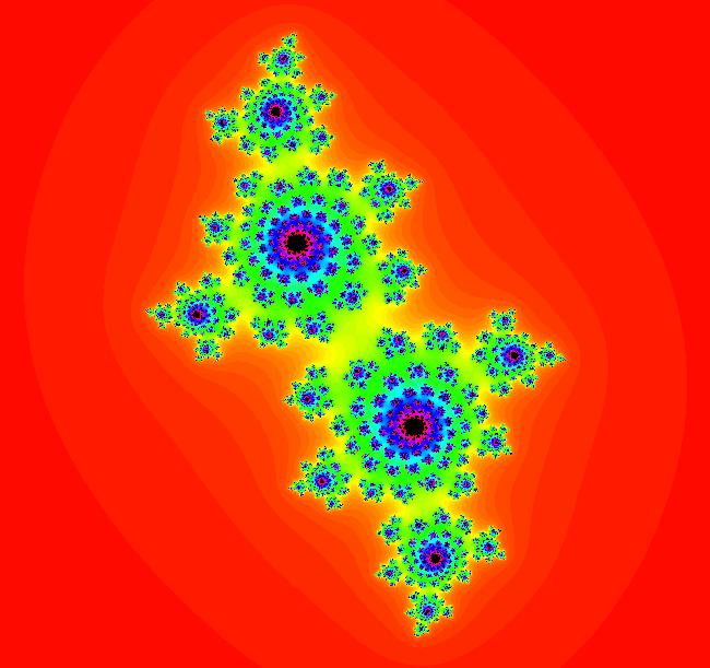
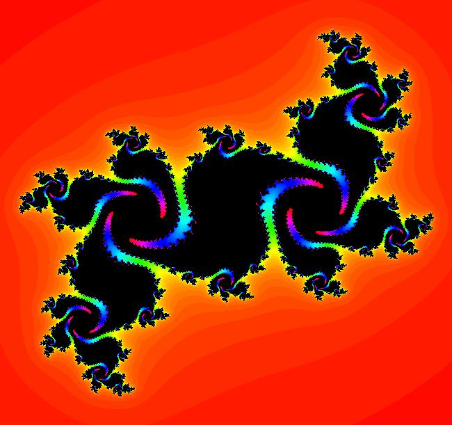
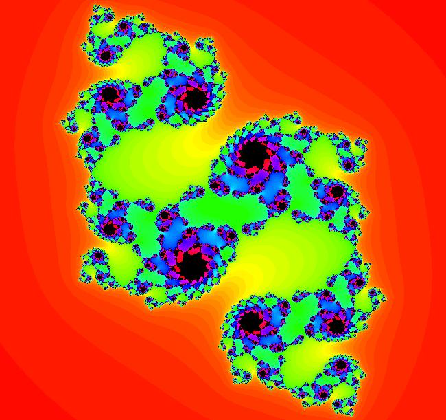
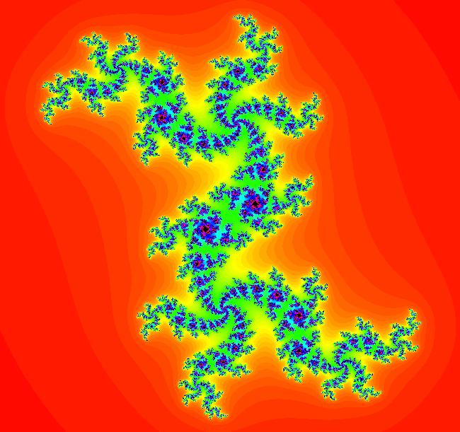
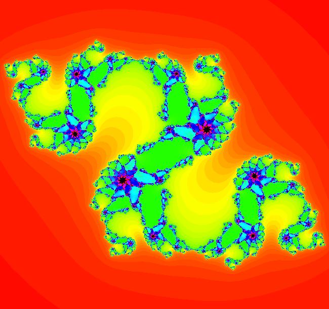
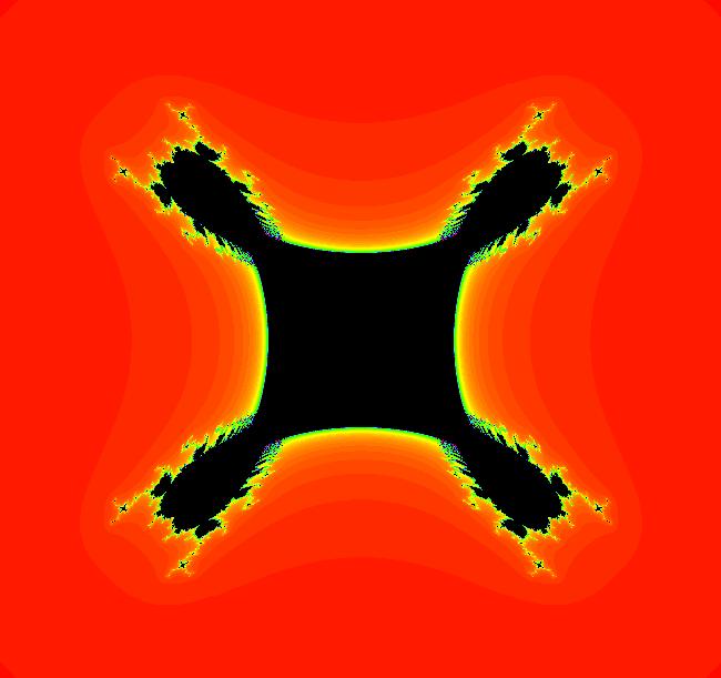
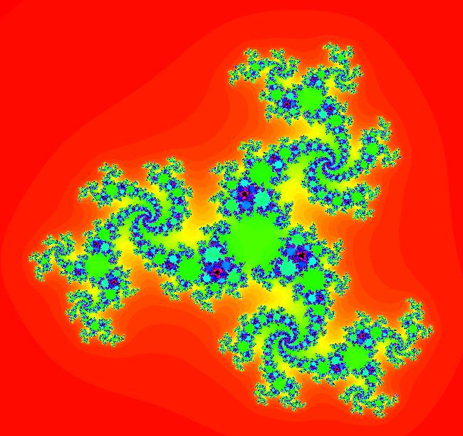
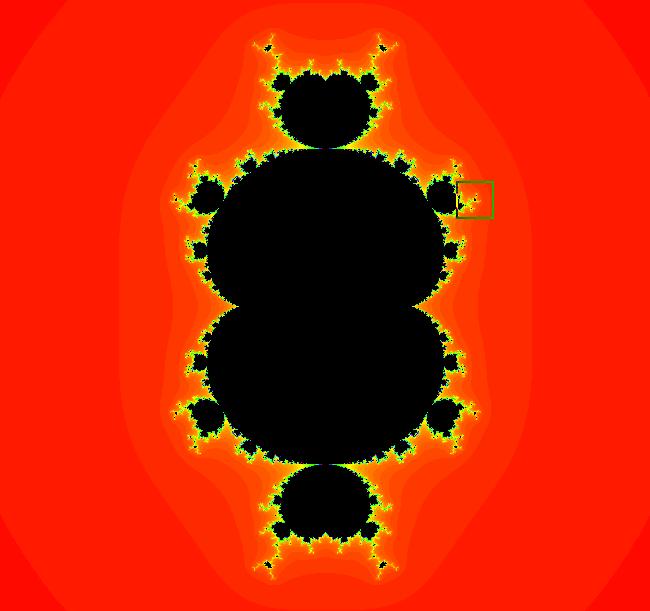
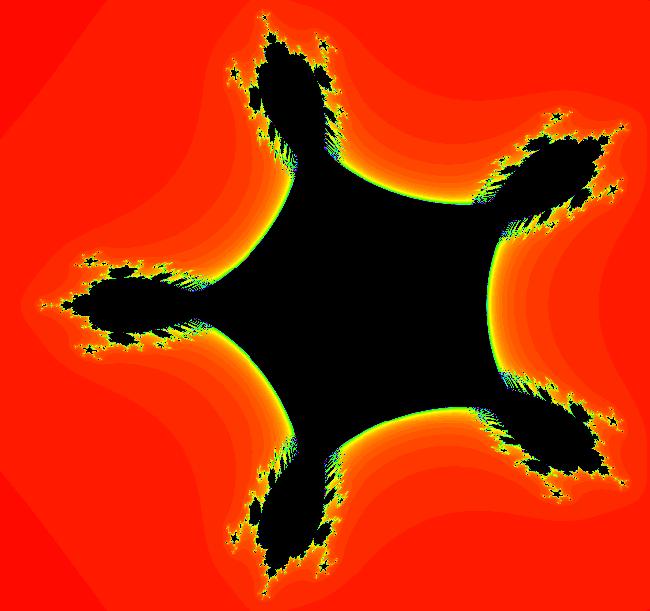
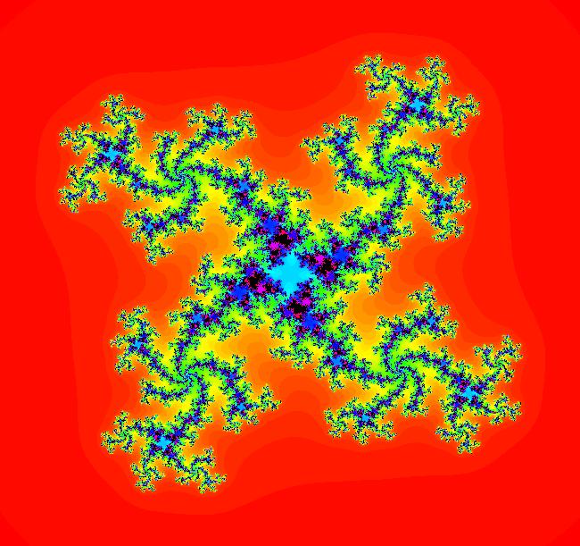
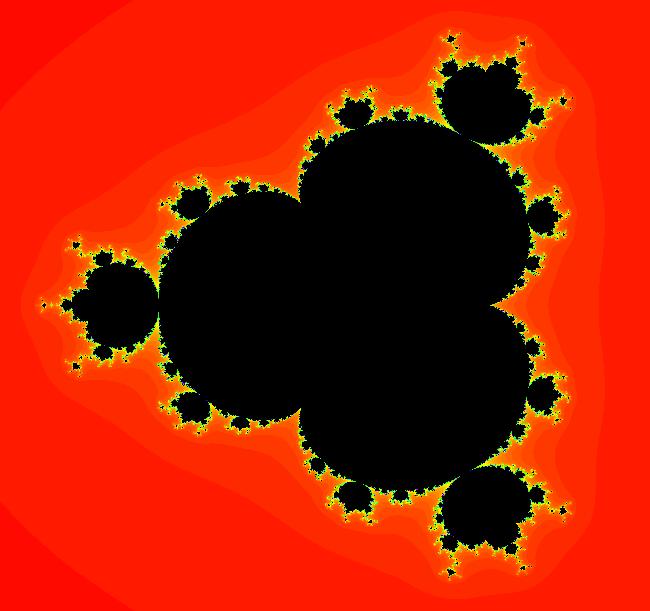
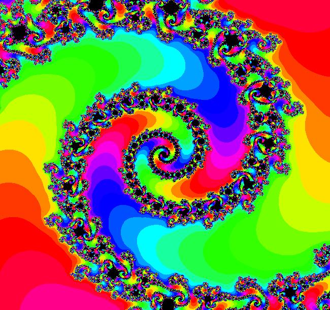
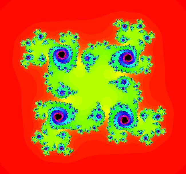
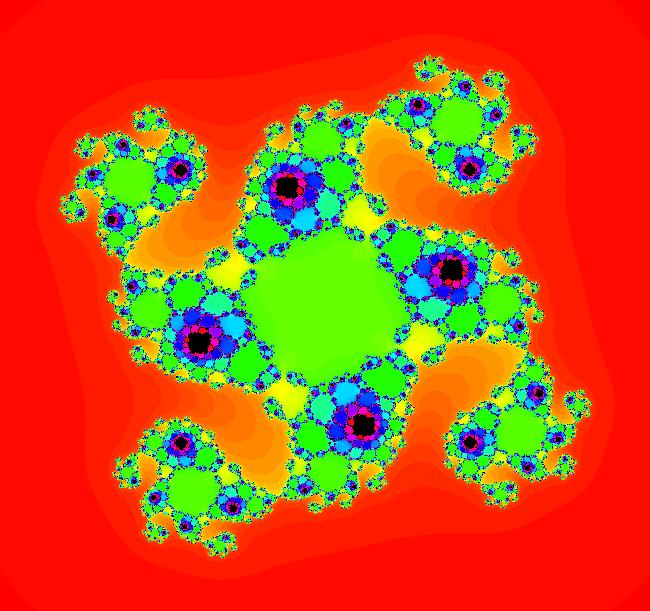
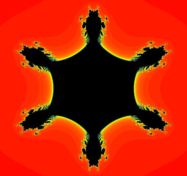
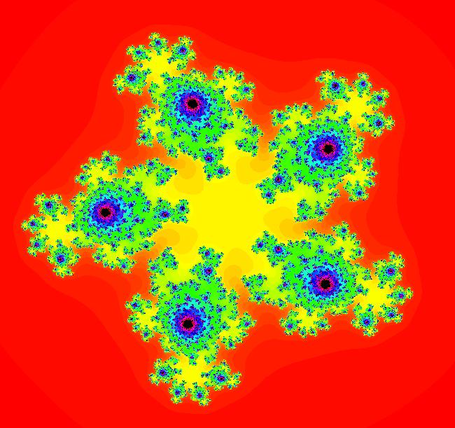
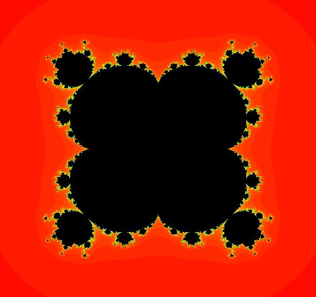
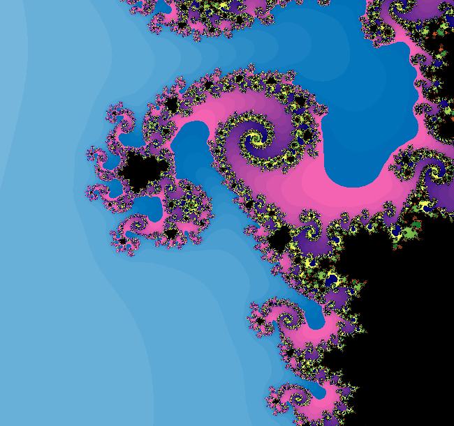
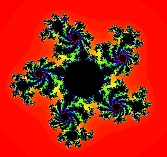
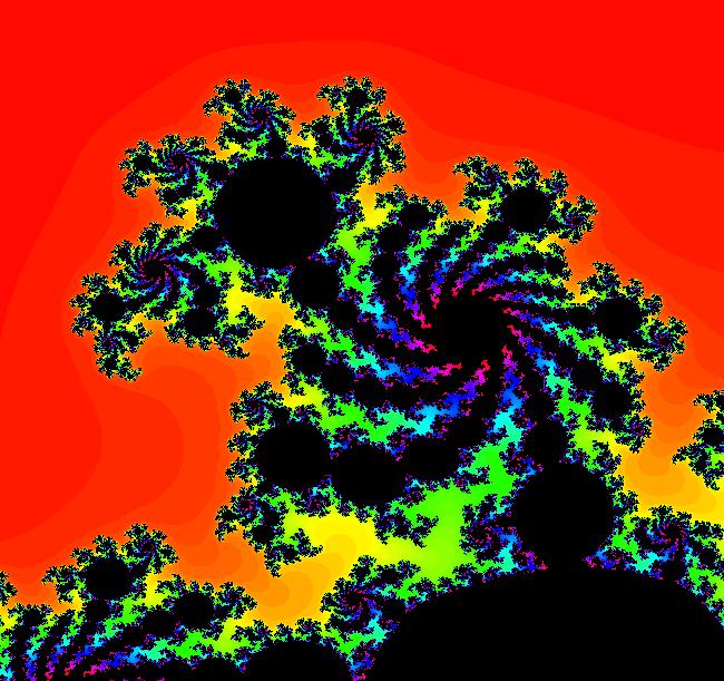
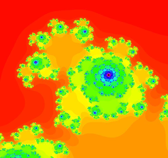
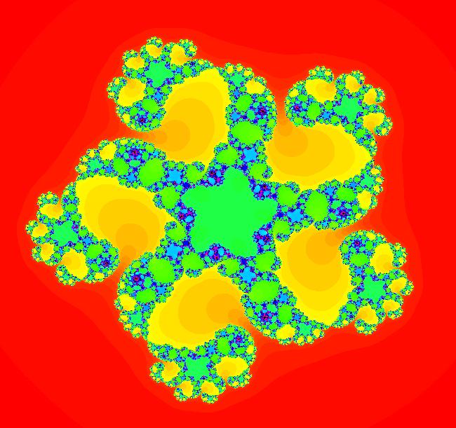
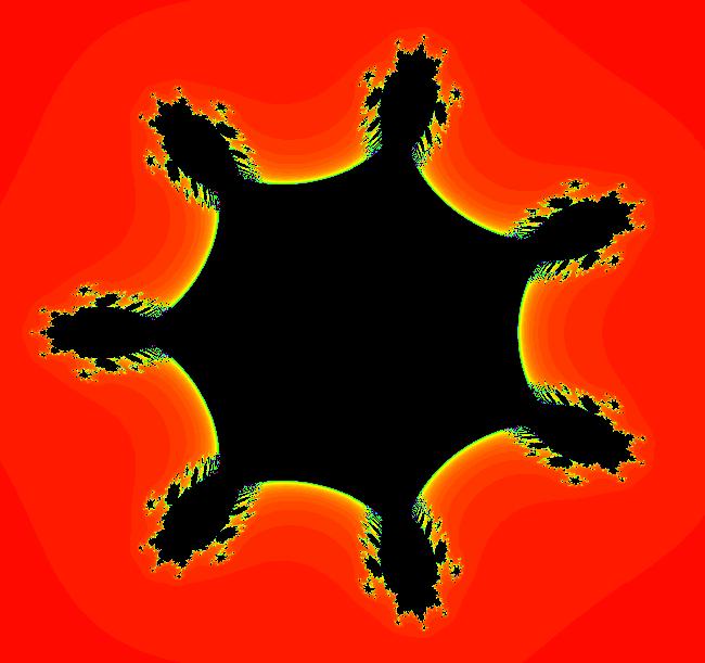
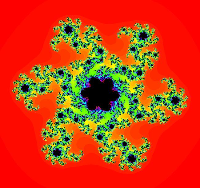
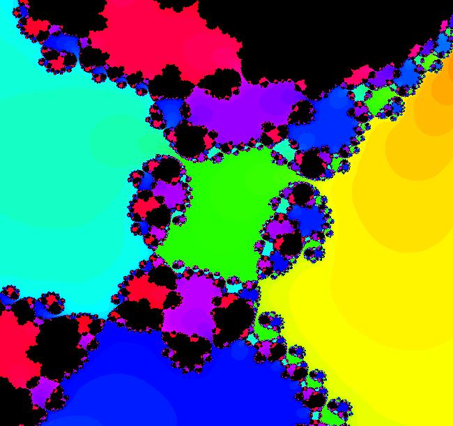
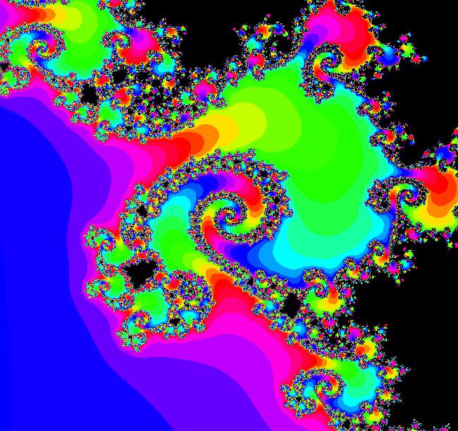
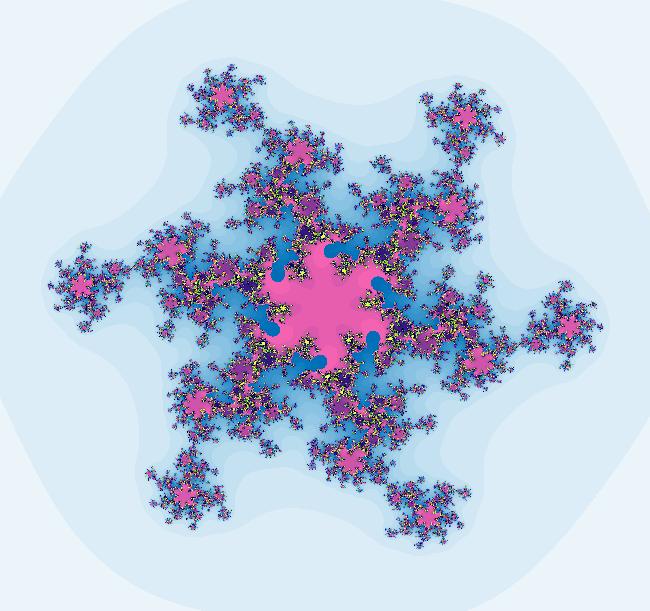
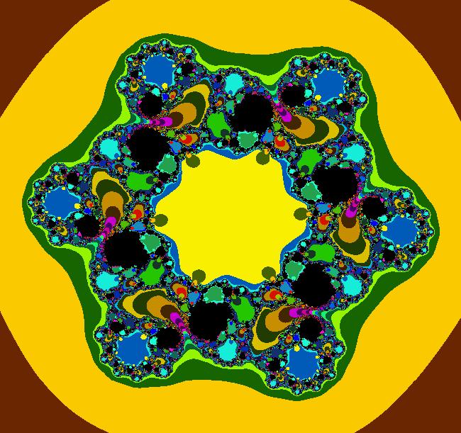
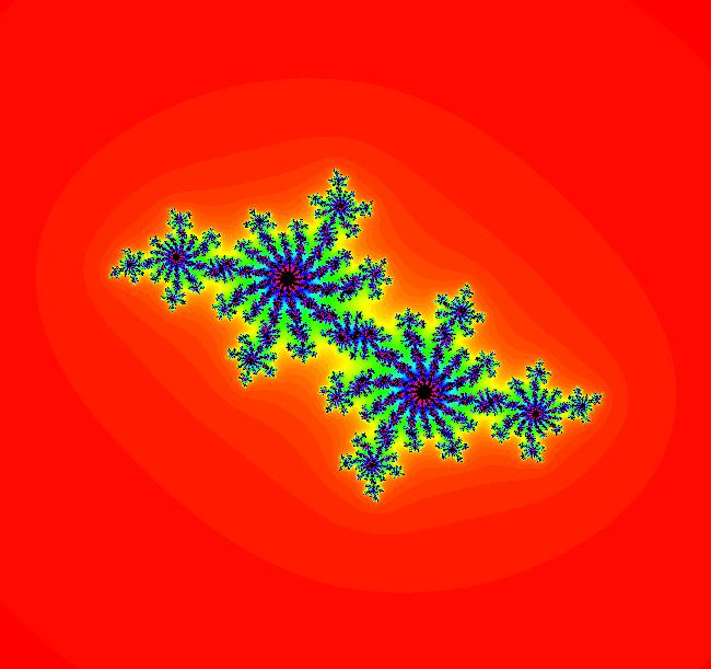
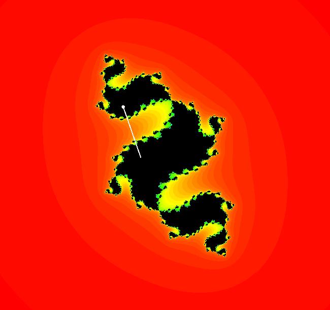
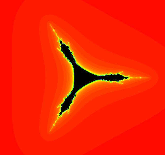
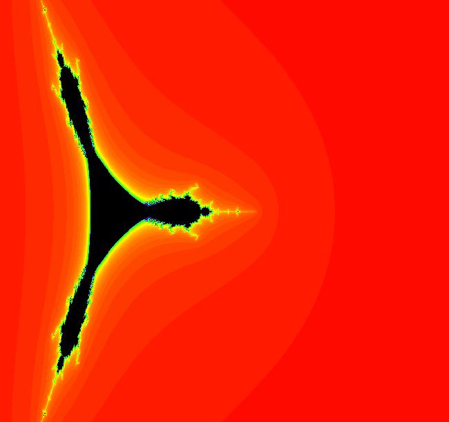
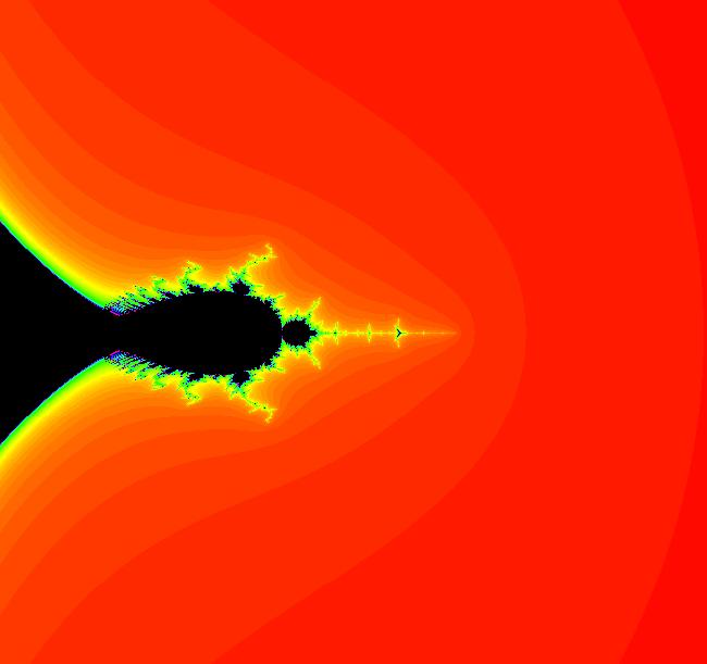
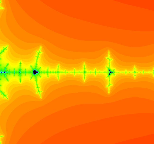
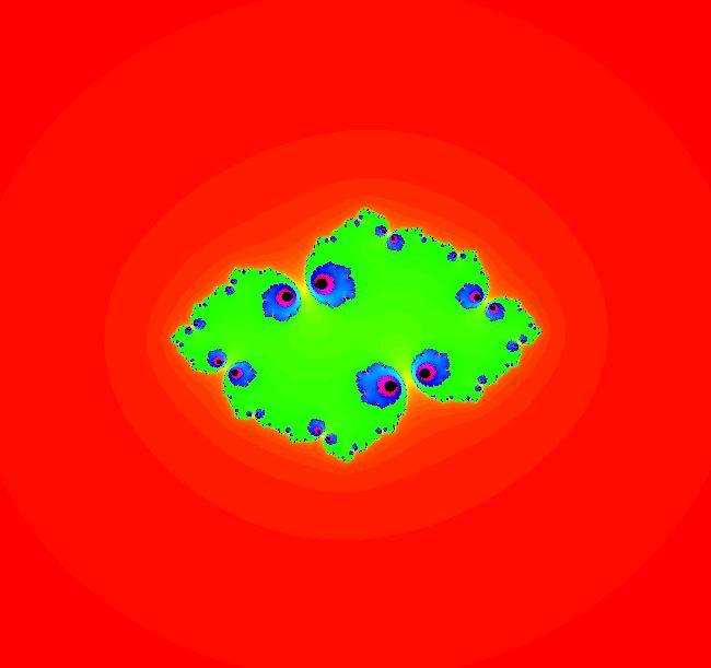
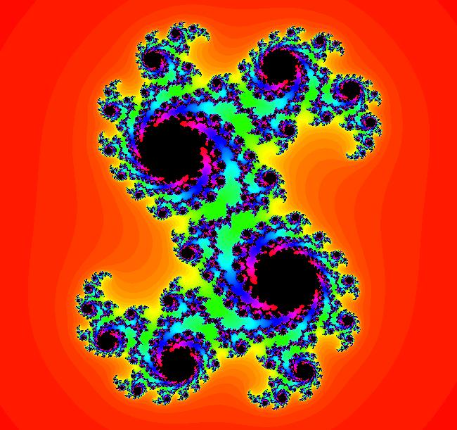
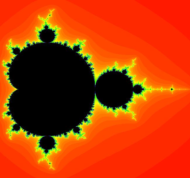
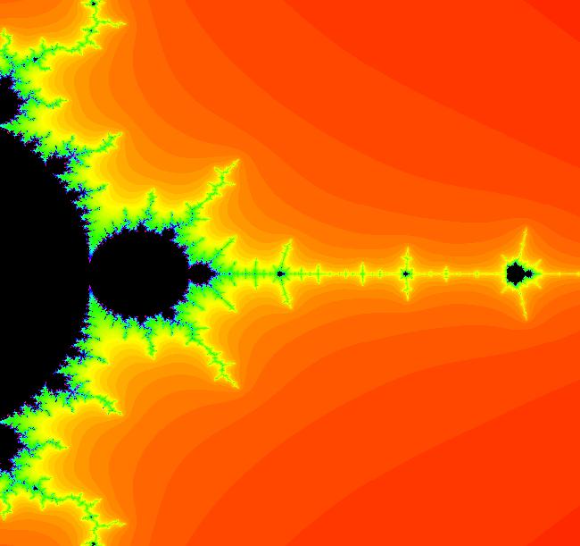
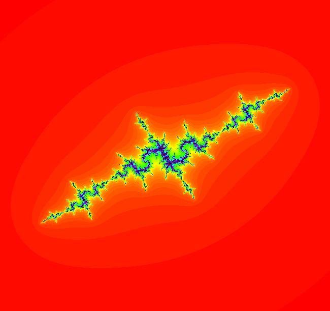
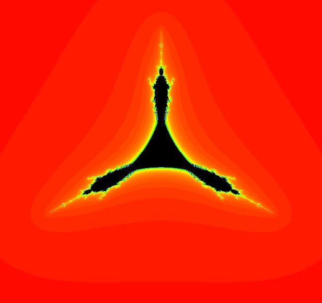
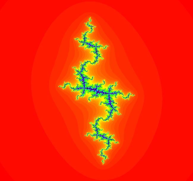
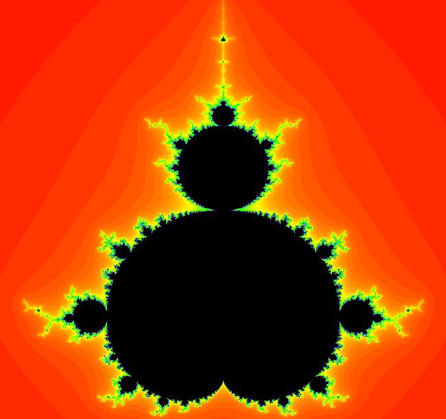
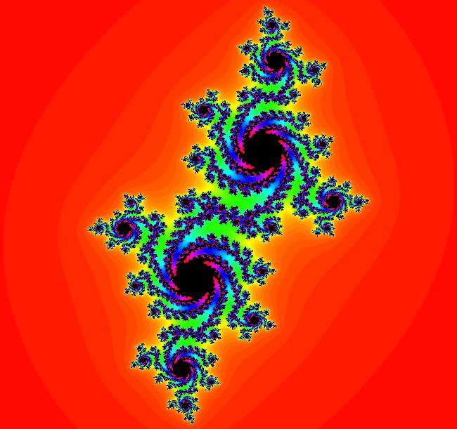
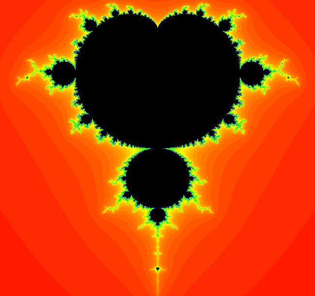
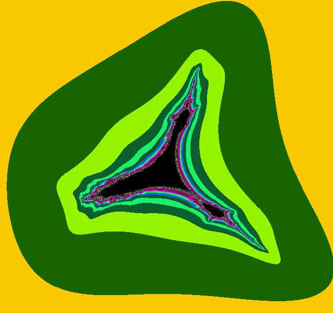
Click on an image to go directly to a system or scroll to see all of the systems in this gallery.
| OdeFactory Images and Annotations |
|
An OdeFactory Slide Show
Click on a slide to zoom in.
Click "video" to see a video. |
View/Sys/Gal: Ode " Introduction to Power Fractals" in "PowerFractals."
Range: (vMax,vMin) = (5.000,-5.000), (hMin,hMax) = (-5.000,5.000)
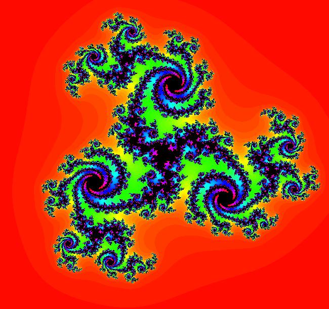
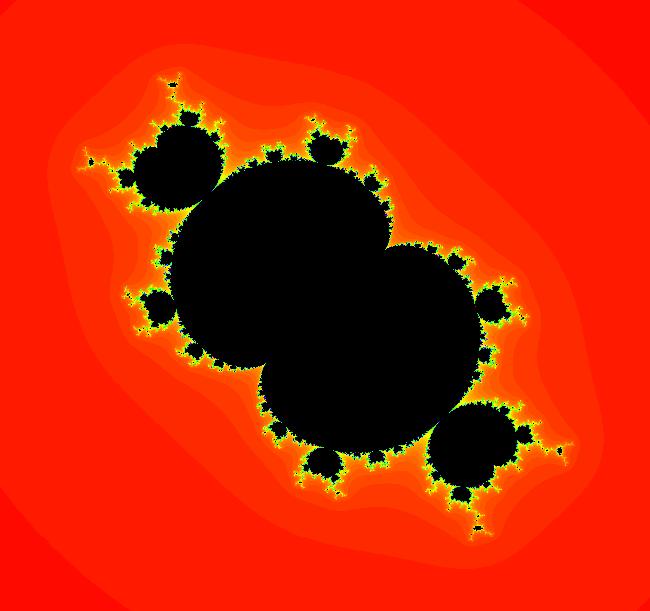
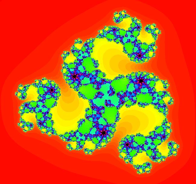
VFld: (0) Introduction to Power Fractals This first section of the gallery discusses power fractals in general. The second section discusses the classic n = 2 case in more detail. Power fractals are generated by the iteration: z <- z^n+c, where z = x+i*y, c = p+i*q, and n = 2, 3, 4, 5, ... The n = 2 case corresponds to the classic Mandelbrot iteration. For each n, enter (x+i*y)^n into WA. and double click on the form that contains a single i term. This will enter it into the WA entry field which will enable you to copy/paste the plain text to any simple text editor. You should then replace each space by a * to get it into proper OdeFactory syntax. In the OdeFactory "user fns:" field enter: F = re(z^n); G = im(z^n) In the "x <-" and "y <-" fields enter: F+p and G+q respectively In the "params:" field enter: p=.5; q=.5 Update the system and get into the EMap view. Adjust p until you get an image (a Julia set) that is not mostly black then adjust q until you get an interesting fractal. Save the system, with EMap in its' name. Examine the EMaps for the related systems x <- G+q y <- F+p and x <- G+q y <- -(F+p) for various values of p and q. The system: x <- F+p, y <- -G+q, corresponds to the iteration z <- conj(z)^n+c which also gives interesting fractals called Mandelbar fractals (since z "bar" is used in place of z). The n = 2 case of the "z <- z^n+c" iteration is the classic Mandelbrot iteration. Since all of the systems z<-z^n+c have 2 state variables and 2 parameters, I call them "2D2P" systems. It is easy (in OdeFactory) to create bifurcation diagrams for 2D2P iterated systems by creating 4D0P companion iterated systems. For n>2 the bifurcation diagrams could be thought of as higher order "Mandelbrot" sets.
|
|

|
View/Sys/Gal: EMap "EMap z^2, (-(G+q),F+p)" in "PowerFractals."
Range: (vMax,vMin) = (1.600,-1.600), (hMin,hMax) = (-1.600,1.600)
VFld: (-(G+q),(F+p)), p = .56; q = .50; , F=x^2-y^2; G=2*x*y This iteration is defined by: x <- -(G+q), y <- (F+p). Parameters are: p = .56; q = .50; Functions are: F=x^2-y^2; G=2*x*y Click "Adj Ctrl Params..." and try changing parameter values and/or color tables.
|
|

|
View/Sys/Gal: EMap "EMap z^2, (-G+q,F+p)" in "PowerFractals."
Range: (vMax,vMin) = (1.250,-1.250), (hMin,hMax) = (-1.250,1.250)
VFld: (-G+q,(F+p)), p = -.24; q = .52; , F=x^2-y^2; G=2*x*y This iteration is defined by: x <- -G+q, y <- (F+p). Parameters are: p = -.24; q = .52; Functions are: F=x^2-y^2; G=2*x*y
|
|

|
View/Sys/Gal: EMap "EMap z^2, (F+p,-G+q)" in "PowerFractals."
Range: (vMax,vMin) = (1.250,-1.250), (hMin,hMax) = (-1.250,1.250)
VFld: (F+p,-G+q), p = .24; q = -.54; , F=x^2-y^2; G=2*x*y This is the Mandelbar system z <- conj(z)^2+c, c = p+i*q. This iteration is defined by: x <- F+p, y <- -G+q. Parameters are: p = .24; q = -.54; Functions are: F=x^2-y^2; G=2*x*y
|
|

|
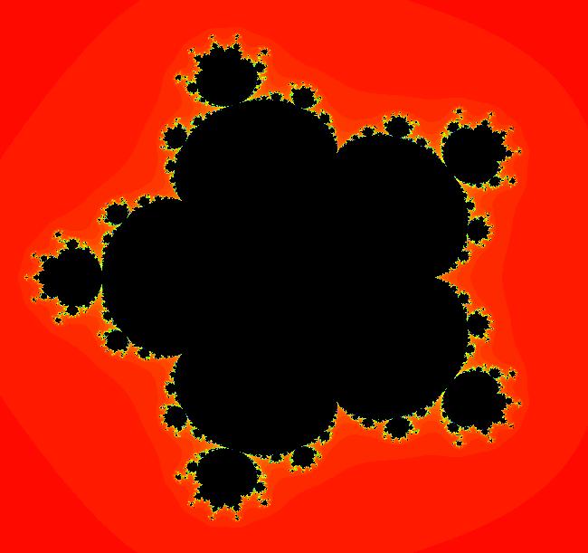
View/Sys/Gal: EMap "EMap z^2, (F+p,G+q)" in "PowerFractals."
Range: (vMax,vMin) = (1.250,-1.250), (hMin,hMax) = (-1.250,1.250)
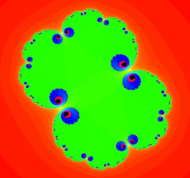
VFld: (F+p,G+q), p = .32; q = .50; , F=x^2-y^2; G=2*x*y This is the classic Mandelbrot iteration z <- z^2+c, c = p+i*q. This iteration is defined by: x <- F+p, y <- G+q. Parameters are: p = .32; q = .50; Functions are: F=x^2-y^2; G=2*x*y The image is called the Julia set for (p,q). Vary p and q to get different Julia sets.
|
|


|
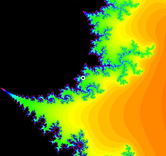
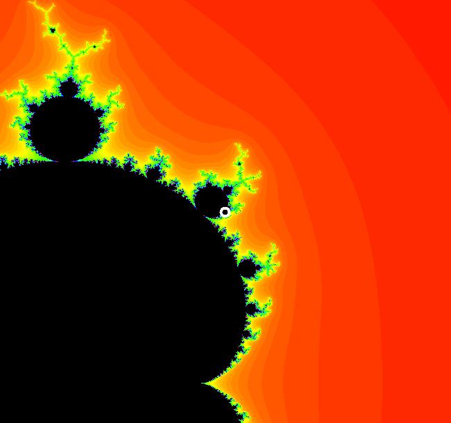
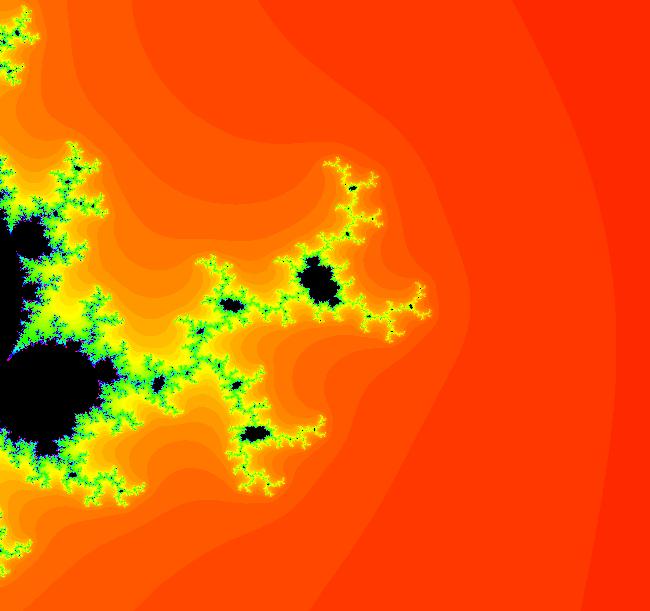
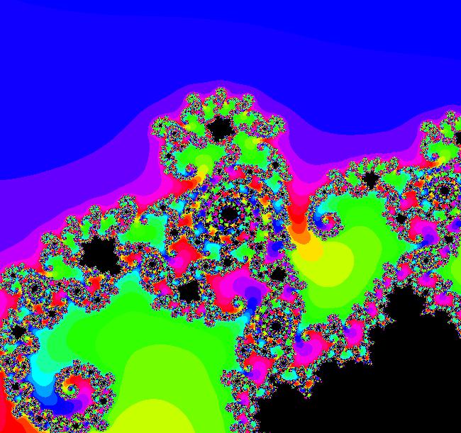
View/Sys/Gal: EMap "EMap z^2, (F+p,G+q) zoomed in at (p,q) = (.32,.5)" in "PowerFractals."
Range: (vMax,vMin) = (1.125,-0.125), (hMin,hMax) = (-0.305,0.945)
VFld: (x,y,z^2-w^2+x,2*z*w+y) This iteration is defined by: x <- x, y <- y, z <- z^2-w^2+x, w <- 2*z*w+y. The image is centered at (x,y) = (p,q) = (.32,.5). Image 1: Start a Flow to see the dot. Image 2: Zoomed out.
|
|

|
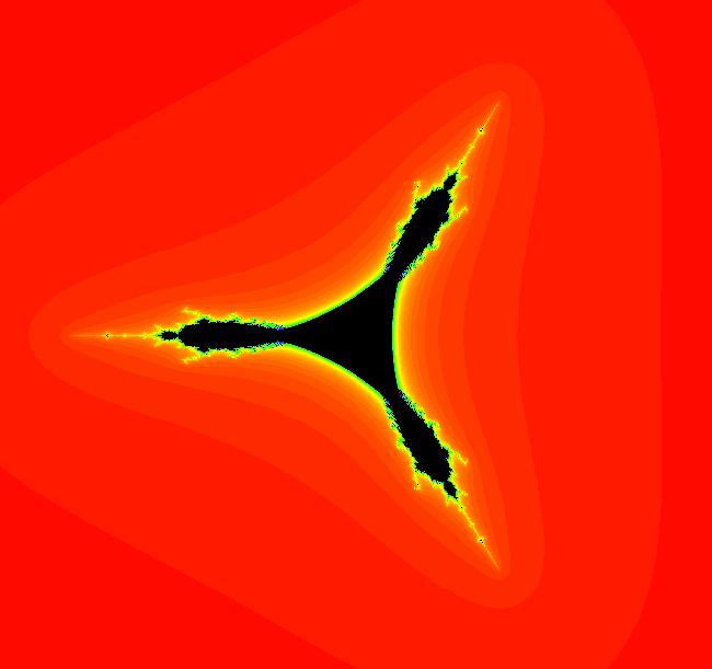
View/Sys/Gal: EMap "EMap z^2, (F,-G)'s bifurcation diagram" in "PowerFractals."
Range: (vMax,vMin) = (2.500,-2.500), (hMin,hMax) = (-2.500,2.500)
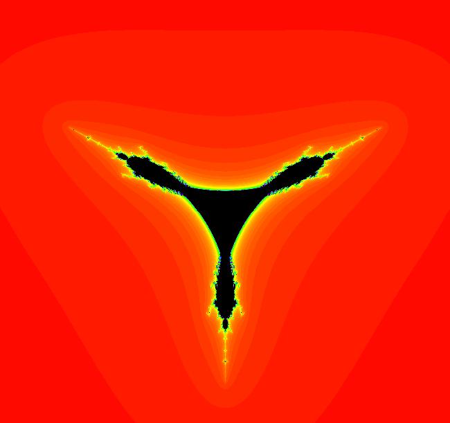
VFld: (x,y,z^2-w^2+x,-2*z*w+y) This iteration is defined by: x <- x, y <- y, z <- z^2-w^2+x, w <- -2*z*w+y. This is sometimes called the Mandelbar set.
|
|

|
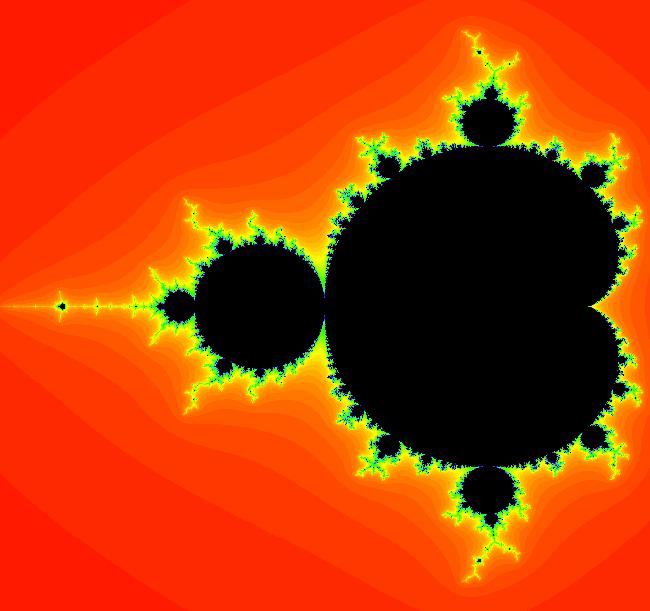
View/Sys/Gal: EMap "EMap z^2, (F,G)'s bifurcation diagram" in "PowerFractals."
Range: (vMax,vMin) = (1.250,-1.250), (hMin,hMax) = (-2.000,0.500)
VFld: (x,y,z^2-w^2+x,2*z*w+y) This iteration is defined by: x <- x, y <- y, z <- z^2-w^2+x, w <- 2*z*w+y. It is the classic Mandelbrot set.
|
|

|
View/Sys/Gal: EMap "EMap z^2, (G+q,-(F+p)) same as (-(G+q),F+p)" in "PowerFractals."
Range: (vMax,vMin) = (1.600,-1.600), (hMin,hMax) = (-1.600,1.600)
VFld: (G+q,-(F+p)), p = .56; q = .50; , F=x^2-y^2; G=2*x*y This iteration is defined by: x <- G+q, y <- -(F+p). Parameters are: p = .56; q = .50; Functions are: F=x^2-y^2; G=2*x*y The system x <- -(G+q), y <- (F+p) gives the same EMap and the trajectories in the Ode view just differ by a time reversal. Change the signs and update to see for yourself.
|
|

|
View/Sys/Gal: EMap "EMap z^2, (G+q,F+p)" in "PowerFractals."
Range: (vMax,vMin) = (1.250,-1.250), (hMin,hMax) = (-1.250,1.250)
VFld: (G+q,F+p), p = -.23; q = .55; , F=x^2-y^2; G=2*x*y This iteration is defined by: x <- G+q, y <- F+p. Parameters are: p = -.23; q = .55; Functions are: F=x^2-y^2; G=2*x*y
|
|

|
View/Sys/Gal: EMap "EMap z^3, (F+p,-G+q)'s bifurcation diagram" in "PowerFractals."
Range: (vMax,vMin) = (1.500,-1.500), (hMin,hMax) = (-1.500,1.500)
VFld: (x,y,z*(z^2-3*w^2)+x,-w*(3*z^2-w^2)+y) This iteration is defined by: x <- x, y <- y, z <- z*(z^2-3*w^2)+x, w <- -w*(3*z^2-w^2)+y.
|
|

|
View/Sys/Gal: EMap "EMap z^3, (F+p,G+q)" in "PowerFractals."
Range: (vMax,vMin) = (1.375,-1.125), (hMin,hMax) = (-1.375,1.125)
VFld: (F+p,G+q), p = .57; q = .31; , F=x*(x^2-3*y^2); G=y*(3*x^2-y^2) This is the iteration z <- z^3+c, c = p+i*q. This iteration is defined by: x <- F+p, y <- G+q. Parameters are: p = .57; q = .31; Functions are: F=x*(x^2-3*y^2); G=y*(3*x^2-y^2)
|
|


|
View/Sys/Gal: EMap "EMap z^3, (F+p,Q+q)'s bifurcation diagram" in "PowerFractals."
Range: (vMax,vMin) = (0.603,0.428), (hMin,hMax) = (0.607,0.773)
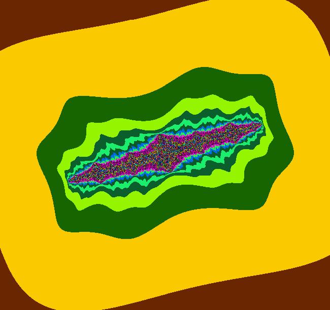
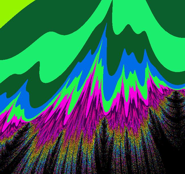
VFld: (x,y,z*(z^2-3*w^2)+x,w*(3*z^2-w^2)+y) This iteration is defined by: x <- x, y <- y, z <- z*(z^2-3*w^2)+x, w <- w*(3*z^2-w^2)+y. This is the bifurcation diagram for the iteration defined by: x <- F+p, y <- G+q, where: F=x*(x^2-3*y^2); G=y*(3*x^2-y^2) Image 1: The entire bifurcation diagram. Zoom in on any of the small black regions to see the fractal nature of the image. Image 2: Zoomed in view.
|
|

|
View/Sys/Gal: EMap "EMap z^3, (G+p,-F+q)" in "PowerFractals."
Range: (vMax,vMin) = (1.250,-1.250), (hMin,hMax) = (-1.250,1.250)
VFld: (G+p,-F+q), p = .26; q = .50; , F=x*(x^2-3*y^2); G=y*(3*x^2-y^2) This iteration is defined by: x <- G+p, y <- -F+q. Parameters are: p = .26; q = .50; Functions are: F=x*(x^2-3*y^2); G=y*(3*x^2-y^2)
|
|

|
View/Sys/Gal: EMap "EMap z^3, (G+p,-F+q)'s bifurcation diagram" in "PowerFractals."
Range: (vMax,vMin) = (1.500,-1.500), (hMin,hMax) = (-1.500,1.500)
VFld: (x,y,w*(3*z^2-w^2)+x,-z*(z^2-3*w^2)+y) This iteration is defined by: x <- x, y <- y, z <- w*(3*z^2-w^2)+x, w <- -z*(z^2-3*w^2)+y. This is just the previous z^3 bifurcation diagram rotated ccw by 45 degrees.
|
|

|
View/Sys/Gal: EMap "EMap z^3, (G+p,F+q)" in "PowerFractals."
Range: (vMax,vMin) = (1.310,-1.190), (hMin,hMax) = (-1.354,1.146)
VFld: (G+p,F+q), p = .31; q = .53; , F=x*(x^2-3*y^2); G=y*(3*x^2-y^2) This iteration is defined by: x <- G+p, y <- F+q. Parameters are: p = .31; q = .53; Functions are: F=x*(x^2-3*y^2); G=y*(3*x^2-y^2)
|
|

|
View/Sys/Gal: EMap "EMap z^4, (F+p,-G+q)'s bifurcation diagram" in "PowerFractals."
Range: (vMax,vMin) = (1.245,-1.255), (hMin,hMax) = (-1.398,1.102)
VFld: (x,y,z^4-6*z^2*w^2+w^4+x,-(4*z^3*w-4*z*w^3)+y) This iteration is defined by: x <- x, y <- y, z <- z^4-6*z^2*w^2+w^4+x, w <- -(4*z^3*w-4*z*w^3)+y.
|
|

|
View/Sys/Gal: EMap "EMap z^4, (F+p,Q+q)" in "PowerFractals."
Range: (vMax,vMin) = (1.250,-1.250), (hMin,hMax) = (-1.250,1.250)
VFld: (F+p,G+q), p = .62; q = .49; , F=x^4-6*x^2*y^2+y^4; G=4*x^3*y-4*x*y^3 This is the iteration z <- z^4+c, c = p+i*q. This iteration is defined by: x <- F+p, y <- G+q. Parameters are: p = .62; q = .49; Functions are: F=x^4-6*x^2*y^2+y^4; G=4*x^3*y-4*x*y^3
|
|


|
View/Sys/Gal: EMap "EMap z^4, (F+p,Q+q)'s bifurcation diagram" in "PowerFractals."
Range: (vMax,vMin) = (0.751,0.749), (hMin,hMax) = (0.318,0.319)
VFld: (x,y,z^4-6*z^2*w^2+w^4+x,4*z^3*w-4*z*w^3+y) This iteration is defined by: x <- x, y <- y, z <- z^4-6*z^2*w^2+w^4+x, w <- 4*z^3*w-4*z*w^3+y. Image 1: The bifurcation diagram. Image 2: Centered at (x,y) = (.31886,.75000), zoomed in 4X with CT1.
|
|

|
View/Sys/Gal: EMap "EMap z^4, (G+q,-(F+p))" in "PowerFractals."
Range: (vMax,vMin) = (1.250,-1.250), (hMin,hMax) = (-1.250,1.250)
VFld: (G+q,-(F+p)), p = .63; q = .39; , F=x^4-6*x^2*y^2+y^4; G=4*x^3*y-4*x*y^3 This iteration is defined by: x <- G+q, y <- -(F+p). Parameters are: p = .63; q = .39; Functions are: F=x^4-6*x^2*y^2+y^4; G=4*x^3*y-4*x*y^3
|
|

|
View/Sys/Gal: EMap "EMap z^4, (G+q,F+p)" in "PowerFractals."
Range: (vMax,vMin) = (1.250,-1.250), (hMin,hMax) = (-1.250,1.250)
VFld: (G+q,F+p), p = .53; q = .49; , F=x^4-6*x^2*y^2+y^4; G=4*x^3*y-4*x*y^3 This iteration is defined by: x <- G+q, y <- F+p. Parameters are: p = .53; q = .49; Functions are: F=x^4-6*x^2*y^2+y^4; G=4*x^3*y-4*x*y^3
|
|

|
View/Sys/Gal: EMap "EMap z^5, (F+p,-G+q)'s bifurcation diagram" in "PowerFractals."
Range: (vMax,vMin) = (1.250,-1.250), (hMin,hMax) = (-1.250,1.250)
VFld: (x,y,z^5-10*z^3*w^2+5*z*w^4+x,-(5*z^4*w-10*z^2*w^3+w^5)+y) This iteration is defined by: x <- x, y <- y, z <- z^5-10*z^3*w^2+5*z*w^4+x, w <- -(5*z^4*w-10*z^2*w^3+w^5)+y.
|
|

|
View/Sys/Gal: EMap "EMap z^5, (F+p,G+q)" in "PowerFractals."
Range: (vMax,vMin) = (1.250,-1.250), (hMin,hMax) = (-1.250,1.250)
VFld: (F+p,G+q), p = .69; q = .37; , F=x^5-10*x^3*y^2+5*x*y^4; G=5*x^4*y-10*x^2*y^3+y^5 This is the iteration z <- z^5+c, c = p+i*q. This iteration is defined by: x <- F+p, y <- G+q. Parameters are: p = .69; q = .37; Functions are: F=x^5-10*x^3*y^2+5*x*y^4; G=5*x^4*y-10*x^2*y^3+y^5
|
|


|
View/Sys/Gal: EMap "EMap z^5, (F+p,G+q)'s bifurcation diagram" in "PowerFractals."
Range: (vMax,vMin) = (0.652,0.640), (hMin,hMax) = (0.510,0.523)
VFld: (x,y,z^5-10*z^3*w^2+5*z*w^4+x,5*z^4*w-10*z^2*w^3+w^5+y) This iteration is defined by: x <- x, y <- y, z <- z^5-10*z^3*w^2+5*z*w^4+x, w <- 5*z^4*w-10*z^2*w^3+w^5+y. Image 1: The bifurcation diagram. Image 2: Centered at (x,y) = (.51674,.64576), zoomed in 3X using CT3.
|
|

|
View/Sys/Gal: EMap "EMap z^5, (G+q,-(F+p))" in "PowerFractals."
Range: (vMax,vMin) = (1.250,-1.250), (hMin,hMax) = (-1.250,1.250)
VFld: (G+q,-(F+p)), p = .57; q = .41; , F=x^5-10*x^3*y^2+5*x*y^4; G=5*x^4*y-10*x^2*y^3+y^5 This iteration is defined by: x <- G+q, y <- -(F+p). Parameters are: p = .57; q = .41; Functions are: F=x^5-10*x^3*y^2+5*x*y^4; G=5*x^4*y-10*x^2*y^3+y^5
|
|

|
View/Sys/Gal: EMap "EMap z^5, (G+q,-(F+p)) ver 2" in "PowerFractals."
Range: (vMax,vMin) = (1.153,0.115), (hMin,hMax) = (-0.763,0.217)
VFld: (G+q,-(F+p)), p = .57; q = .41; , F=x^5-10*x^3*y^2+5*x*y^4; G=5*x^4*y-10*x^2*y^3+y^5 This iteration is defined by: x <- G+q, y <- -(F+p). Parameters are: p = .57; q = .41; Functions are: F=x^5-10*x^3*y^2+5*x*y^4; G=5*x^4*y-10*x^2*y^3+y^5
|
|

|
View/Sys/Gal: EMap "EMap z^5, (G+q,-(F+p)) ver 2, time-scaled" in "PowerFractals."
Range: (vMax,vMin) = (1.153,0.115), (hMin,hMax) = (-0.763,0.217)
VFld: ((1+s*.01)*(G+q),-(1+s*.01)*(F+p)), p = .57; q = .41; s=1, F=x^5-10*x^3*y^2+5*x*y^4; G=5*x^4*y-10*x^2*y^3+y^5 This iteration is defined by: x <- (1+s*.01)*(G+q), y <- -(1+s*.01)*(F+p). Parameters are: p = .57; q = .41; s=1 Functions are: F=x^5-10*x^3*y^2+5*x*y^4; G=5*x^4*y-10*x^2*y^3+y^5 This is the time-scaled version of the previous system. Time-scaling can be used to reduce the size of the basins of attraction (the black regions). Try decreasing s from 1 to 0.
|
|

|
View/Sys/Gal: EMap "EMap z^5, (G+q,F+p)" in "PowerFractals."
Range: (vMax,vMin) = (1.250,-1.250), (hMin,hMax) = (-1.250,1.250)
VFld: (G+q,F+p), p = .52; q = .37; , F=x^5-10*x^3*y^2+5*x*y^4; G=5*x^4*y-10*x^2*y^3+y^5 This iteration is defined by: x <- G+q, y <- F+p. Parameters are: p = .52; q = .37; Functions are: F=x^5-10*x^3*y^2+5*x*y^4; G=5*x^4*y-10*x^2*y^3+y^5
|
|

|
View/Sys/Gal: EMap "EMap z^6, (F+p,-G+q)'s bifurcation diagram" in "PowerFractals."
Range: (vMax,vMin) = (1.250,-1.250), (hMin,hMax) = (-1.250,1.250)
VFld: (x,y,z^6-15*z^4*w^2+15*z^2*w^4-w^6+x,-(6*z^5*w-20*z^3*w^3+6*z*w^5)+y) This iteration is defined by: x <- x, y <- y, z <- z^6-15*z^4*w^2+15*z^2*w^4-w^6+x, w <- -(6*z^5*w-20*z^3*w^3+6*z*w^5)+y.
|
|

|
View/Sys/Gal: EMap "EMap z^6, (F+p,G+q)" in "PowerFractals."
Range: (vMax,vMin) = (1.250,-1.250), (hMin,hMax) = (-1.250,1.250)
VFld: (F+p,G+q), p = -.62; q = .36; , F=x^6-15*x^4*y^2+15*x^2*y^4-y^6; G=6*x^5*y-20*x^3*y^3+6*x*y^5 This is the iteration z <- z^6+c, c = p+i*q. This iteration is defined by: x <- F+p, y <- G+q. Parameters are: p = -.62; q = .36; Functions are: F=x^6-15*x^4*y^2+15*x^2*y^4-y^6; G=6*x^5*y-20*x^3*y^3+6*x*y^5
|
|


|
View/Sys/Gal: EMap "EMap z^6, (F+p,G+q)'s bifurcation diagram" in "PowerFractals."
Range: (vMax,vMin) = (0.542,0.540), (hMin,hMax) = (0.616,0.617)
VFld: (x,y,z^6-15*z^4*w^2+15*z^2*w^4-w^6+x,6*z^5*w-20*z^3*w^3+6*z*w^5+y) This iteration is defined by: x <- x, y <- y, z <- z^6-15*z^4*w^2+15*z^2*w^4-w^6+x, w <- 6*z^5*w-20*z^3*w^3+6*z*w^5+y. Image 1: The bifurcation diagram. Image 2: Centered at (x,y) = (.61637,.54105), zoomed in 4X with CT1.
|
|

|
View/Sys/Gal: EMap "EMap z^6, (G+q,-(F+p))" in "PowerFractals."
Range: (vMax,vMin) = (1.250,-1.250), (hMin,hMax) = (-1.250,1.250)
VFld: (G+q,-(F+p)), p = .62; q = .36; , F=x^6-15*x^4*y^2+15*x^2*y^4-y^6; G=6*x^5*y-20*x^3*y^3+6*x*y^5 This iteration is defined by: x <- G+q, y <- -(F+p). Parameters are: p = .62; q = .36; Functions are: F=x^6-15*x^4*y^2+15*x^2*y^4-y^6; G=6*x^5*y-20*x^3*y^3+6*x*y^5
|
|

|
View/Sys/Gal: EMap "EMap z^6, (G+q,-(F+p)) ver 2" in "PowerFractals."
Range: (vMax,vMin) = (1.250,-1.250), (hMin,hMax) = (-1.250,1.250)
VFld: (G+q,-(F+p)), p = .50; q = .38; , F=x^6-15*x^4*y^2+15*x^2*y^4-y^6; G=6*x^5*y-20*x^3*y^3+6*x*y^5 This iteration is defined by: x <- G+q, y <- -(F+p). Parameters are: p = .50; q = .38; Functions are: F=x^6-15*x^4*y^2+15*x^2*y^4-y^6; G=6*x^5*y-20*x^3*y^3+6*x*y^5
|
|

|
View/Sys/Gal: EMap "EMap z^6, (G+q,F+p)" in "PowerFractals."
Range: (vMax,vMin) = (1.250,-1.250), (hMin,hMax) = (-1.250,1.250)
VFld: (G+q,F+p), p = -.62; q = .36; , F=x^6-15*x^4*y^2+15*x^2*y^4-y^6; G=6*x^5*y-20*x^3*y^3+6*x*y^5 This iteration is defined by: x <- G+q, y <- F+p. Parameters are: p = -.62; q = .36; Functions are: F=x^6-15*x^4*y^2+15*x^2*y^4-y^6; G=6*x^5*y-20*x^3*y^3+6*x*y^5
|
|

|
View/Sys/Gal: EMap "EMap z^6, (G+q,F+p) ver 2" in "PowerFractals."
Range: (vMax,vMin) = (0.149,-0.209), (hMin,hMax) = (0.335,0.675)
VFld: (G+q,F+p), p = -.62; q = .36; , F=x^6-15*x^4*y^2+15*x^2*y^4-y^6; G=6*x^5*y-20*x^3*y^3+6*x*y^5 This iteration is defined by: x <- G+q, y <- F+p. Parameters are: p = -.62; q = .36; Functions are: F=x^6-15*x^4*y^2+15*x^2*y^4-y^6; G=6*x^5*y-20*x^3*y^3+6*x*y^5 This one is a bit slow to draw. It should probably be time-scaled, starting with s = 0.
|
|

|
View/Sys/Gal: EMap "EMapCT1 z^4+c: (F+p,G+q)'s bifurcation diagram again" in "PowerFractals."
Range: (vMax,vMin) = (0.756,0.744), (hMin,hMax) = (0.313,0.325)
VFld: (x,y,z^4-6*z^2*w^2+w^4+x,4*z^3*w-4*z*w^3+y) This system is defined by the iterations: x <- x, y <- y, z <- z^4-6*z^2*w^2+w^4+x, w <- 4*z^3*w-4*z*w^3+y. Zoomed in.
|
|

|
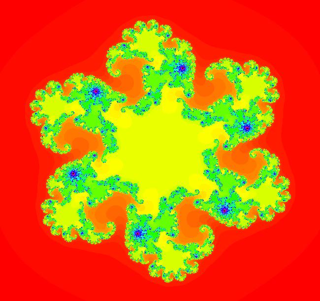
View/Sys/Gal: EMap "EMapCT3 z^6, XMass 2014 Snow Flake" in "PowerFractals."
Range: (vMax,vMin) = (1.250,-1.250), (hMin,hMax) = (-1.250,1.250)
VFld: ((1+s*.1)*(G+q),(1+s*.1)*(F+p)), p = -.610; q = .360; s = 3.100; , F=x^6-15*x^4*y^2+15*x^2*y^4-y^6; G=6*x^5*y-20*x^3*y^3+6*x*y^5 This iteration is defined by: x <- (1+s*.1)*(G+q), y <- (1+s*.1)*(F+p). Parameters are: p = -.610; q = .360; s = 3.100; Functions are: F=x^6-15*x^4*y^2+15*x^2*y^4-y^6; G=6*x^5*y-20*x^3*y^3+6*x*y^5 EMap CT: 3 Parameter s is a time-scaling parameter used to reduce the amount of black in the image.
|
|

|
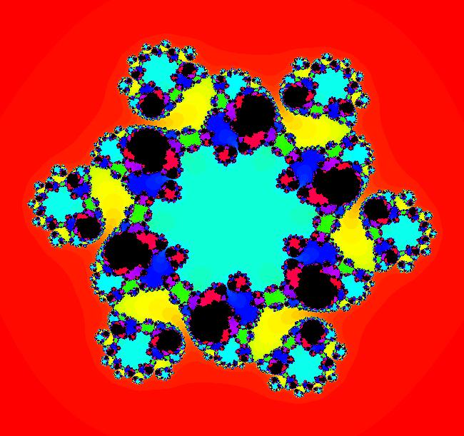
View/Sys/Gal: EMap "EMapCT5 z^6, XMass 2014 Wreath" in "PowerFractals."
Range: (vMax,vMin) = (1.250,-1.250), (hMin,hMax) = (-1.250,1.250)
VFld: ((1+s*.1)*(G+q),(1+s*.1)*(F+p)), p = -.620; q = .360; s = .002; , F=x^6-15*x^4*y^2+15*x^2*y^4-y^6; G=6*x^5*y-20*x^3*y^3+6*x*y^5 This iteration is defined by: x <- (1+s*.1)*(G+q), y <- (1+s*.1)*(F+p). Parameters are: p = -.620; q = .360; s = .002; Functions are: F=x^6-15*x^4*y^2+15*x^2*y^4-y^6; G=6*x^5*y-20*x^3*y^3+6*x*y^5 EMap CT: 5 Also try CT 3.
|
|
An OdeFactory Slide Show
Click on a slide to zoom in.
Click "video" to see a video. |
View/Sys/Gal: Ode "z^2+c: Bifurcation Diagrams" in "PowerFractals."
Range: (vMax,vMin) = (5.000,-5.000), (hMin,hMax) = (-5.000,5.000)
VFld: (0) This section of the gallery shows the bifurcation diagrams of variations of the 2D2P iterative system "z <- z^2+c," for z and c complex. Eight variations of the vector field: V = (F,G) = (x^2-y^2,2*x*y), given by, (1) (F,G) (5) (G,F)* (2) (-F,G)* (6) (-G,F) (3) (F.-G)* (7) (G,-F) (4) (-F,-G) (8) (-G,-F)* are considered. The variations with an asterisk give a 3-sided variation of the classic Mandelbrot set with a 120 degree rotational symmetry. The classic Mandelbrot set is symmetric about the long axis. Bifurcation diagrams 1, 4, 6 and 7 are topologically the same and are the Mandelbrot set. Bifurcation diagrams 2, 3, 5 and 8 are topologically the same and are the Mandelbar set (they use z bar in place of z in the iteration). The Mandelbar set contains regions quasi-similar to itself and to the Mandelbrot set. See systems: z^2+c: (2Mbar) EMap tail and z^2+c: (4M) EMap tail
|
|

|
View/Sys/Gal: EMap "z^2+c: (1J) (F,G) EMap" in "PowerFractals."
Range: (vMax,vMin) = (2.000,-2.000), (hMin,hMax) = (-2.000,2.000)
VFld: (F+p,G+q), p = -.420; q = .600; , F=x^2-y^2; G=2*x*y This iteration is defined by: x <- F+p, y <- G+q. Parameters are: p = -.420; q = .600; Functions are: F=x^2-y^2; G=2*x*y EMap CT: 0
|
|

|
View/Sys/Gal: EMap "z^2+c: (1M) EMap" in "PowerFractals."
Range: (vMax,vMin) = (1.250,-1.250), (hMin,hMax) = (-2.000,0.500)
VFld: (x,y,a*F+b*G+x,c*G+d*F+y), a=1; b=0; c=1; d=0, F=z^2-w^2; G=2*z*w This system is defined by the iterations: x <- x, y <- y, z <- a*F+b*G+x, w <- c*G+d*F+y. Parameters are: a=1; b=0; c=1; d=0 Functions are: F=z^2-w^2; G=2*z*w (x,y) = (p,q) = (-.42,.6) Start a Flow to see (p,q). Zoom in at (p,q).
|
|

|
View/Sys/Gal: EMap "z^2+c: (2J) (-F,G) EMap" in "PowerFractals."
Range: (vMax,vMin) = (2.000,-2.000), (hMin,hMax) = (-2.000,2.000)
VFld: (-F+p,G+q), p = -.420; q = .600; , F=x^2-y^2; G=2*x*y This iteration is defined by: x <- -F+p, y <- G+q. Parameters are: p = -.420; q = .600; Functions are: F=x^2-y^2; G=2*x*y EMap CT: 0 The black region is a basin of attraction. The attractor is the 2-cycle shown by the white line.
|
|

|
View/Sys/Gal: EMap "z^2+c: (2Mbar) EMap" in "PowerFractals."
Range: (vMax,vMin) = (2.500,-2.500), (hMin,hMax) = (-2.500,2.500)
VFld: (x,y,a*F+b*G+x,c*G+d*F+y), a=-1; b=0; c=1; d=0, F=z^2-w^2; G=2*z*w This system is defined by the equations: x <- x, y <- y, z <- a*F+b*G+x, w <- c*G+d*F+y. Parameters are: a=-1; b=0; c=1; d=0 Functions are: F=z^2-w^2; G=2*z*w (x,y) = (p,q) = (-.42,.6) Start a Flow to see (p,q). Zoom in at (p,q).
|
|


|
View/Sys/Gal: EMap "z^2+c: (2Mbar) EMap tail" in "PowerFractals."
Range: (vMax,vMin) = (0.080,-0.080), (hMin,hMax) = (1.408,1.712)
VFld: (x,y,a*F+b*G+x,c*G+d*F+y), a=-1; b=0; c=1; d=0, F=z^2-w^2; G=2*z*w This system is defined by the equations: x <- x, y <- y, z <- a*F+b*G+x, w <- c*G+d*F+y. Parameters are: a=-1; b=0; c=1; d=0 Functions are: F=z^2-w^2; G=2*z*w This is a series of zoomed-in images. Image 1: Initial image. Image 2: Image 1 zoomed in 1X. Image 3: Image 2 zoomed in 1X. In image 3, the small black region on the left is quasi-similar to the Mandelbrot set and the small right most black region is quasi-similar to the Mbar set itself.
|
|

|
View/Sys/Gal: EMap "z^2+c: (3J) (F,-G) EMap" in "PowerFractals."
Range: (vMax,vMin) = (2.500,-2.500), (hMin,hMax) = (-2.500,2.500)
VFld: (F+p,-G+q), p = -.400; q = .100; , F=x^2-y^2; G=2*x*y This iteration is defined by: x <- F+p, y <- -G+q. Parameters are: p = -.400; q = .100; Functions are: F=x^2-y^2; G=2*x*y EMap CT: 0
|
|

|
View/Sys/Gal: EMap "z^2+c: (3Mbar) EMap" in "PowerFractals."
Range: (vMax,vMin) = (2.500,-2.500), (hMin,hMax) = (-2.500,2.500)
VFld: (x,y,a*F+b*G+x,c*G+d*F+y), a=1; b=0; c=-1; d=0, F=z^2-w^2; G=2*z*w This system is defined by the iterations: x <- x, y <- y, z <- a*F+b*G+x, w <- c*G+d*F+y. Parameters are: a=1; b=0; c=-1; d=0 Functions are: F=z^2-w^2; G=2*z*w (x,y) = (p,q) = (-.4,.1) Start a Flow to see (p,q). Zoom in at (p,q).
|
|

|
View/Sys/Gal: EMap "z^2+c: (4J) (-F,-G) EMap" in "PowerFractals."
Range: (vMax,vMin) = (1.250,-1.250), (hMin,hMax) = (-1.250,1.250)
VFld: (-F+p,-G+q), p = -.360; q = .110; , F=x^2-y^2; G=2*x*y This iteration is defined by: x <- -F+p, y <- -G+q. Parameters are: p = -.360; q = .110; Functions are: F=x^2-y^2; G=2*x*y EMap CT: 0
|
|

|
View/Sys/Gal: EMap "z^2+c: (4M) EMap" in "PowerFractals."
Range: (vMax,vMin) = (1.250,-1.250), (hMin,hMax) = (-0.500,2.000)
VFld: (x,y,a*F+b*G+x,c*G+d*F+y), a=-1; b=0; c=-1; d=0, F=z^2-w^2; G=2*z*w This system is defined by the iterations: x <- x, y <- y, z <- a*F+b*G+x, w <- c*G+d*F+y. Parameters are: a=-1; b=0; c=-1; d=0 Functions are: F=z^2-w^2; G=2*z*w (x,y) = (p,q) = (-.36,.11) Start a Flow to see (p,q). Zoom in at (p,q).
|
|

|
View/Sys/Gal: EMap "z^2+c: (4M) EMap tail" in "PowerFractals."
Range: (vMax,vMin) = (0.388,-0.388), (hMin,hMax) = (1.144,1.836)
VFld: (x,y,a*F+b*G+x,c*G+d*F+y), a=-1; b=0; c=-1; d=0, F=z^2-w^2; G=2*z*w This system is defined by the iterations: x <- x, y <- y, z <- a*F+b*G+x, w <- c*G+d*F+y. Parameters are: a=-1; b=0; c=-1; d=0 Functions are: F=z^2-w^2; G=2*z*w
|
|

|
View/Sys/Gal: EMap "z^2+c: (5J) (G,F) EMap" in "PowerFractals."
Range: (vMax,vMin) = (2.000,-2.000), (hMin,hMax) = (-2.000,2.000)
VFld: (G+p,F+q), p=-1.099; q=-.672, F=x^2-y^2; G=2*x*y This iteration is defined by: x <- G+p, y <- F+q. Parameters are: p=-1.099; q=-.672 Functions are: F=x^2-y^2; G=2*x*y EMap CT: 0
|
|

|
View/Sys/Gal: EMap "z^2+c: (5Mbar) EMap" in "PowerFractals."
Range: (vMax,vMin) = (2.500,-2.500), (hMin,hMax) = (-2.500,2.500)
VFld: (x,y,a*F+b*G+x,c*G+d*F+y), a=0; b=1; c=0; d=1, F=z^2-w^2; G=2*z*w This system is defined by the iterations: x <- x, y <- y, z <- a*F+b*G+x, w <- c*G+d*F+y. Parameters are: a=0; b=1; c=0; d=1 Functions are: F=z^2-w^2; G=2*z*w (x,y) = (p,q) = (-1.099,-.672) Start a Flow to see (p,q). Zoom in at (p,q).
|
|

|
View/Sys/Gal: EMap "z^2+c: (6J) (-G,F) EMap" in "PowerFractals."
Range: (vMax,vMin) = (2.000,-2.000), (hMin,hMax) = (-2.000,2.000)
VFld: (-G+p,F+q), p = -.290; q = 1.000; , F=x^2-y^2; G=2*x*y This iteration is defined by: x <- -G+p, y <- F+q. Parameters are: p = -.290; q = 1.000; Functions are: F=x^2-y^2; G=2*x*y EMap CT: 0
|
|

|
View/Sys/Gal: EMap "z^2+c: (6M) EMap" in "PowerFractals."
Range: (vMax,vMin) = (2.000,-0.500), (hMin,hMax) = (-1.250,1.250)
VFld: (x,y,a*F+b*G+x,c*G+d*F+y), a=0; b=-1; c=0; d=1, F=z^2-w^2; G=2*z*w This system is defined by the iterations: x <- x, y <- y, z <- a*F+b*G+x, w <- c*G+d*F+y. Parameters are: a=0; b=-1; c=0; d=1 Functions are: F=z^2-w^2; G=2*z*w (x,y) = (p,q) = (-.29,1) Start a Flow to see (p,q). Zoom in at (p,q).
|
|

|
View/Sys/Gal: EMap "z^2+c: (7J) (G,-F) EMap" in "PowerFractals."
Range: (vMax,vMin) = (1.500,-1.500), (hMin,hMax) = (-1.500,1.500)
VFld: (G+p,-F+q), p = -.440; q = -.600; , F=x^2-y^2; G=2*x*y This iteration is defined by: x <- G+p, y <- -F+q. Parameters are: p = -.440; q = -.600; Functions are: F=x^2-y^2; G=2*x*y EMap CT: 0
|
|

|
View/Sys/Gal: EMap "z^2+c: (7M) EMap" in "PowerFractals."
Range: (vMax,vMin) = (0.500,-2.000), (hMin,hMax) = (-1.250,1.250)
VFld: (x,y,a*F+b*G+x,c*G+d*F+y), a=0; b=1; c=0; d=-1, F=z^2-w^2; G=2*z*w This system is defined by the iterations: x <- x, y <- y, z <- a*F+b*G+x, w <- c*G+d*F+y. Parameters are: a=0; b=1; c=0; d=-1 Functions are: F=z^2-w^2; G=2*z*w (x,y) = (p,q) = (-.44,-.6) Start a Flow to see (p,q). Zoom in at (p,q).
|
|

|
View/Sys/Gal: EMap "z^2+c: (8J) (-G,-F) EMap" in "PowerFractals."
Range: (vMax,vMin) = (1.250,-1.250), (hMin,hMax) = (-1.250,1.250)
VFld: (-G+p,-F+q), p = -.220; q = -.140; , F=x^2-y^2; G=2*x*y This iteration is defined by: x <- -G+p, y <- -F+q. Parameters are: p = -.220; q = -.140; Functions are: F=x^2-y^2; G=2*x*y EMap CT: 0
|
|

|
View/Sys/Gal: EMap "z^2+c: (8Mbar) EMap" in "PowerFractals."
Range: (vMax,vMin) = (2.500,-2.500), (hMin,hMax) = (-2.500,2.500)
VFld: (x,y,a*F+b*G+x,c*G+d*F+y), a=0; b=-1; c=0; d=-1, F=z^2-w^2; G=2*z*w This system is defined by the iterations: x <- x, y <- y, z <- a*F+b*G+x, w <- c*G+d*F+y. Parameters are: a=0; b=-1; c=0; d=-1 Functions are: F=z^2-w^2; G=2*z*w (x,y) = (p,q) = (-.22,-.14) Start a Flow to see (p,q). Zoom in at (p,q).
|
|

|
View/Sys/Gal: EMap "z^2+c: (9J) (a*F+b*G,c*G+d*F) EMapCT5" in "PowerFractals."
Range: (vMax,vMin) = (2.230,-2.300), (hMin,hMax) = (-2.070,2.070)
VFld: (a*F+b*G+p,c*G+d*F+q), a = 1.000; b = 1.000; c = -.500; d = 1.000; p=-1.1; q=-.368, F=x^2-y^2; G=2*x*y This iteration is defined by: x <- a*F+b*G+p, y <- c*G+d*F+q. Parameters are: a = 1.000; b = 1.000; c = -.500; d = 1.000; p=-1.1; q=-.368 Functions are: F=x^2-y^2; G=2*x*y EMap CT: 5 Zoom in and vary the parameters.
|
|

|
View/Sys/Gal: EMap "z^2+c: (9Jtrees) EMapCT5" in "PowerFractals."
Range: (vMax,vMin) = (0.513,0.143), (hMin,hMax) = (0.105,0.414)
VFld: (a*F+b*G+p,c*G+d*F+q), a = 1.200; b = .800; c = -.500; d = 1.000; p = -1.100; q = -.370; , F=x^2-y^2; G=2*x*y This iteration is defined by: x <- a*F+b*G+p, y <- c*G+d*F+q. Parameters are: a = 1.200; b = .800; c = -.500; d = 1.000; p = -1.100; q = -.370; Functions are: F=x^2-y^2; G=2*x*y EMap CT: 5
|
|

|
View/Sys/Gal: EMap "z^2+c: (9Mvar) (a*F+b*G,c*G+d*F) EMapCT5" in "PowerFractals."
Range: (vMax,vMin) = (2.750,-2.250), (hMin,hMax) = (-2.500,2.500)
VFld: (x,y,a*F+b*G+x,c*G+d*F+y), a = 1.000; b = 1.000; c = -.500; d = 1.000; , F=z^2-w^2; G=2*z*w In this example, the Mandelbrot and Mandelbar sets are mixed. By varying parameters a, b, c and d you can go from one to the other. This system is defined by the iterations: x <- x, y <- y, z <- a*F+b*G+x, w <- c*G+d*F+y. Parameters are: a = 1.000; b = 1.000; c = -.500; d = 1.000; Functions are: F=z^2-w^2; G=2*z*w Try varying the parameters.
|
