AGFs

Algebraically Generated Flows

by

Jerry Tutsch, Copyright © 2/13/01

Consider the flow in R² defined by the solutions to the differential equations

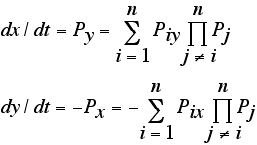
which may also be written as

The local and global properties of the flow are traditionally arrived at by studying explicit solutions to the initial value problem and/or by studying local and/or global properties of the functions f and g.

In the simplest nontrivial case, where f and g are homogeneous linear functions of x and y, the system is generally written as

The topologically distinct flows defined by this simple system can be classified using the properties of the eigenvalues and eigenvectors of the (constant) coefficient matrix A. When the eigenvalues are real and distinct, the eigenvectors are in the directions of the separatrices of the system and the eigenvalues determine the rate of the flow on the separatrices. The separatrices themselves are straight lines through the origin.

In this document I propose a different approach to studying the properties of class of flows in R² based more on synthesis and less on analysis. The idea is to begin by defining a set of special solution curves, which will generally turn out to be separatrices, and rates on these special curves, and then study the flow generated by the set of curves.

I call a flow in R² that has a given algebraic curve, P(x,y) = 0, among its solutions, an algebraically generated flow. The curve can always be written as a product of its irreducible components in the complex field as

For the sake of simplicity let us assume that

P(x,y) has no multiple components,
that each component has real points and
that complex components occur in conjugate pairs

The first order system of ordinary differential equations

has P(x,y) = c as its general solution. If we generalize this system to

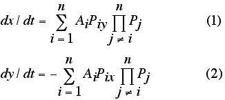
where not all of the A_i's are equal, then it is easy to see that P(x,y) = 0 is a solution to the new system, that is, the n components of P are among the solution curves to equations (1) and (2). Equations (1) and (2) constitute the least complex (lowest degree) nontrivial system for which P(x,y) = 0 is a solution. I call the system of equations given by (1) and (2) the master equation. Flows given by the master equation are generated by P(x,y). The irreducible components of P(x,y) are called the generators of the flow.

The non zero constant coefficients, A_i, in the master equation are called the global rates. They are related to another set of parameters

called the local rates. The relationship between the global rates and the local rates, in the case that each P_i is a linear function, are given by

where c_iand b_i are real but a_iand b_i may be real or complex, is defined by

When the generators of the flow are linear, requiring dx/dt and dy/dt to be real forces A_i and A_j to be complex conjugates if P_i and P_jare complex conjugates. The local rates of the system are the eigenvalues of the linearized system at isolated critical points lying on exactly two generators and the two generators are in the directions of the corresponding eigenvectors.

To define a linearly generated flow in R² using the master equation given by equations (1) and (2), simply specify a set of real and complex lines, of the form given in equation (3), and the local rate on each line at its center, (c_i, d_i).

The system of odes given by equations (1) and (2) is nonlinear when more than two linear generators are involved, consequently a computer is needed to study nontrivial AGFs. Go to OdeFactory.com for a free copy of OdeFactory which, in addition to being a general purpose ode development environment, allows you to create and study AGFs by entering and editing generators and local rates directly. If for some reason you want to see the right hand sides of equations (1) and (2) as polynomials in x and y, OdeFactory will show them to you. The program uses the form shown in (1) and (2) to compute solution curves internally.

It should be noted that in the more general case where P(x,y) is not algebraic, the components of P(x,y) are still solutions to equations (1) and (2). Furthermore, when all of the A_is equal 1, equations (1) and (2) become a Hamiltonian system.

Examples of AGFs are given in sample galleries: AGFExamples, TwoComplexLines, QuasiHamiltonian, AGFEMapExs, AGFFractals and AGFs&Mandelbrot.

In 1973 I wrote a book called "Algebraically Generated Flows." At that time access to computers that could do fast graphics was essentially nonexistent. Interesting AGFs are highly nonlinear so they are difficult to study without a computer. Consequently I never tried to publish the book. In 2000 I started to write OdeFactory to study AGFs. The program was expanded to include traditional forms of odes. I scanned the manuscript of the book to pdf files and put it on the web - in case anyone is interested in AGFs.

Here are the links to the pdf files:

TitlePage/Preface/TOC: the title page, the preface and the table of contents.
Chapter1: "Algebraically Generated Flows," pages 1 through 37.
Chapter2: "Real Linear Generators," pages 38 through 80.
Chapter3: "Limit Flows," pages 81 through 109.
Chapter4: "Modifications of the Master Equation," pages 110 through 131.
Chapter5: "Complex Linear Generators," pages 132 through 168.
Chapter6: "Real and Complex Linear Generators," pages 169 through 215.
Chapter7: "Further Conclusions and Some Problems for Future Research," pages 216 through 253.
Appendix:
- Appendix I: "Homogeneous Systems in R2+," pages 254 through 259.
- Appendix II: "Necklace Combinatorics," pages 260 through 271.
- Appendix III: "Computer Program for Plotting Trajectories in R2 or R2+," pages 254 through 285.
References: a list of references used in writing the book, pages 286 through 292.
Notation and Index: a list of notation used in the book plus the index for the book, pages 293 through 297.

The 273 line program was written in BASIC and was executed on a remote timesharing machine connected via a telephone line. The input/output device was a teletype with a paper tape for storing programs and a long roll of 8.5 inch paper. The right hand sides of odes were entered directly into the program. The graphics output consisted of letters and digits printed at rows and columns locations, acting like really big "pixels," on the long roll of paper.

A Sample run of the program is shown on page 281. It is the R2 view of figure 3.3 on page 89 of the book. Bring up gallery AGFExamples in OdeFactory and select the system. Switch to the R2+ view to see figure 3.3 on page 89 reproduced - about 40 years later.

The pdf files total 105 MB.The page numbers in the index are for the entire book so to find a page you need to find the correct chapter then scroll through pages until you find the desired page of the book.