Click on an image to go directly to a system or scroll to see all of the systems in this gallery.
 |
 |
 |
 |
 |
 |
 |
 |
 |
 |
 |
 |
 |
 |
 |
 |
 |
 |
 |
 |
 |
 |
 |
 |
 |
 |
 |
 |
 |
 |
 |
 |
 |
 |
 |
 |
 |
 |
 |
 |
 |
 |
 |
 |
 |
 |
 |
 |
 |
 |
 |
 |
 |
 |
 |
 |
 |
 |
 |
 |
 |
 |
 |
 |
 |
 |
 |
 |
 |
 |
 |
 |
 |
 |
 |
 |
 |
 |
 |
 |
 |
 |
 |
 |
 |
 |
 |
 |
 |
 |
 |
 |
 |
 |
 |
 |
 |
 |
 |
 |
 |
 |
 |
 |
 |
 |
 |
 |
 |
 |
 |
 |
 |
 |
 |
 |
 |
 |
 |
 |
 |
 |
 |
 |
 |
 |
 |
 |
 |
 |
 |
 |
 |
 |
 |
| OdeFactory Images and Annotations | |
|
An OdeFactory Slide Show Click on a slide to zoom in. Click "video" to see a video. |
View/Sys/Gal: Ode " Five Ways to Plot Functions & Curves" in "PlottingCurves." OdeFactory is generally used to display and study nameless curves generated by motion in a vector field. vector field + OdeFactory -> plot of nameless curve It can also be used to plot and study named curves by creating an associated vector field. named curve -> associated vector field + OdeFactory -> plot of named curve. ***** Case 1: y = f(x). This is the general case. f(x) can be smooth or not smooth and may have parameters. No ICs are used to plot the curve. To plot y = f(x) use the system: dx/dt = f(x), w/"S On". The associated vector field is: V(x) = (f(x)). Ex 1: Plot y = abs(a*sin(b*x+c)) using: dx/dt = abs(a*sin(b*x+c)), a = b = 1, c = 0, w/"S On," no ICs. ***** Case 2a: y = f(x), f smooth, no parameters. To plot y = f(x) let: dx/dt = 1, dy/dt = df/dx, w/ICs on y = f(x). The associated vector field is: V(x,y) = (1,df/dx). The vector field defines a family of curves. The ICs are used to select a particular member of the family. Ex 2: Plot y = sin(x), using dx/dt = 1, dy/dt = cos(x), w/ICs (0,0). ***** Case 2b: x = f(t), integrate f'. To integrate f(t)' on [a,b] plot f using: dx/dt = f', w/ICs (a,x(a)), hMax = b, close Bdr to get x(b) then ∫ f' = x(b)-x(a). Here the relationship between RK4 and Simpson's rule is being used. See the "MoreExs" section for details.
Ex 2e: Plot f(t) = sin(t) on I = [1,2] and find the integral of f'(t) = cos(t) on I using: dx/dt = cos(t), w/ICs (1,sin(1)), hMax = 2, ∫ cos(t) on [1,2] = x(2)-x(1) ***** Case 3: H(x,y) = c, H smooth. To plot the curve defined by H(x,y) = c, for H differentiable in x and y, use: dx/dt = ∂H/ ∂y, dy/dt = - ∂H/ ∂x, w/ICs on H(x,y) = c. Here the Hamiltonian system associated with the curve is being used. The vector field is: V(x,y) = ( ∂H/ ∂y,- ∂H/ ∂x). H is called "an integral" of the motion or an "integral curve." Ex 3: Plot x^2+y^2 = 1 using H = x^2+y^2 dx/dt = 2*y, dy/dt = -2*x, w/ICs (1,0). ***** Case 4: Functions defined by integrals. Most functions are nameless and can only be defined by integrals. x(t) = ∫ f(t,x,y) dt, y(t) = ∫ g(t,x,y) dt. The associated vector field is: V(t,x,y) = (f(t,x,y),g(t,x,y)). To plot x(t) and y(t) use: dx/dt = f(t,x,y), dy/dt = g(t,x,y). Setting an IC at (x(0),y(0)) in the plane selects a particular curve. To view x(t) and y(t) use the 3D/(t,x) and 3D/(t,y) views or start trajectories in the (t,x) and (t,y) directly. Ex 4: To plot the Euler spiral that is defined by: C(t) = ∫ cos(t^2) dt and S(t) = ∫ sin(t^2) dt use dx/dt = cos(t^2), dy/dt = sin(t^2), w/ICs: (x(0),y(0)) = (0,0). The 3D/(t,x) view is C(t) and the 3D/(t,y) view is S(t). ***** Case 5: Using WolframAlpha You can also plot functions/curves in WA by simply entering "plot whatever." Examples are: plot y = abs(sin(x), plot y = sin(x), plot x^2+y^2 = 1, plot C(x) and plot (C(x),S(x)). Using WA is easy but it does not automatically generate parameter controllers so for "Ex 1" you cannot watch what happens to the curve y = abs(a*sin(b*x+c)) as you vary a, b and/or c as you can in OdeFactory. Ex 5: Plot C(t) and S(t) using WA. Open WA from the Help menu then copy/paste the following line into WA: plot (C(x),S(x)) Also try WA on: plot y = abs(a*sin(b*x+c)) for a=1, b=1, c=0 To vary a, b and/or c you need to enter new values in the WA entry field and click the "compute" button.
|
|
|
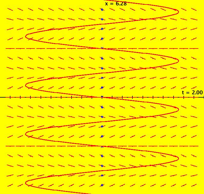
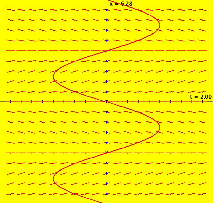
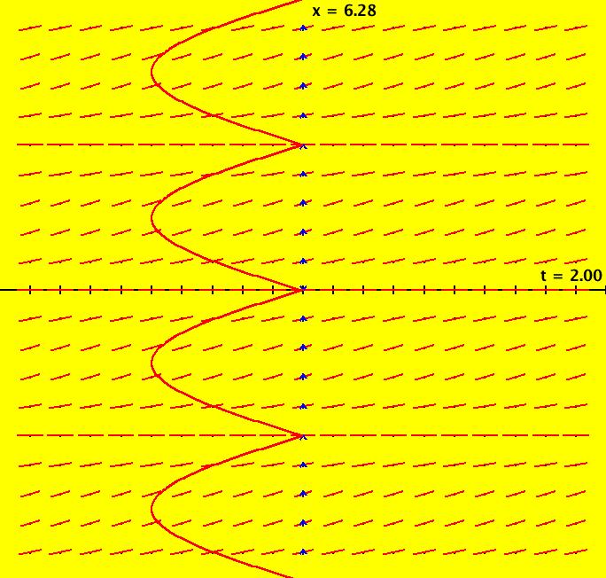
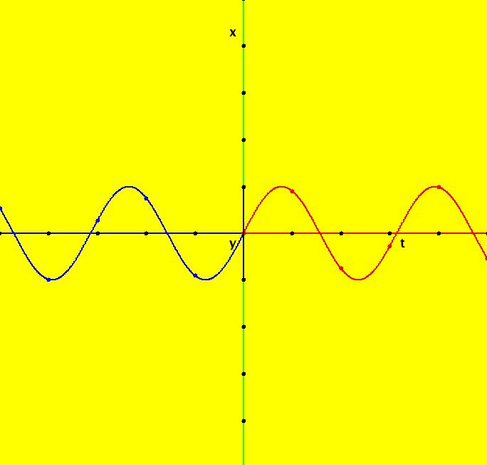
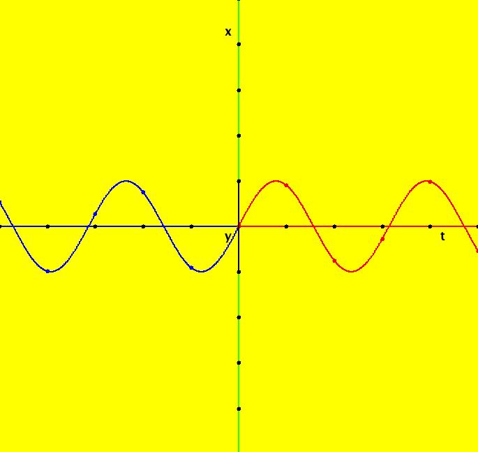
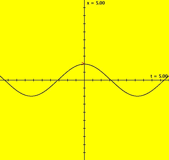
View/Sys/Gal: Ode "Ex 1: y = a*sin(b*x+c), a=1; b=1; c=0" in "PlottingCurves." Case 1: y = f(x), f smooth or not smooth, with or without parameters. This ode is defined by the equation: dx/dt = a*sin(b*x+c) in the (t,x) coordinate system. Parameters are: a=1; b=1; c=0 The red curve about the x axis is "y = f(x)" rotated π/2 ccw (counter clockwise). No ICs are used. As you change a, b and/or c the curve changes correctly. Image 1: y = a*sin(b*x+c), a=1.5; b=2; c=1. Image 2: y = a*sin(b*x+c), a=1; b=1; c=0.
|
|
|
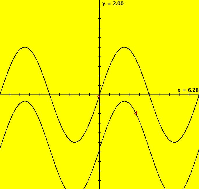
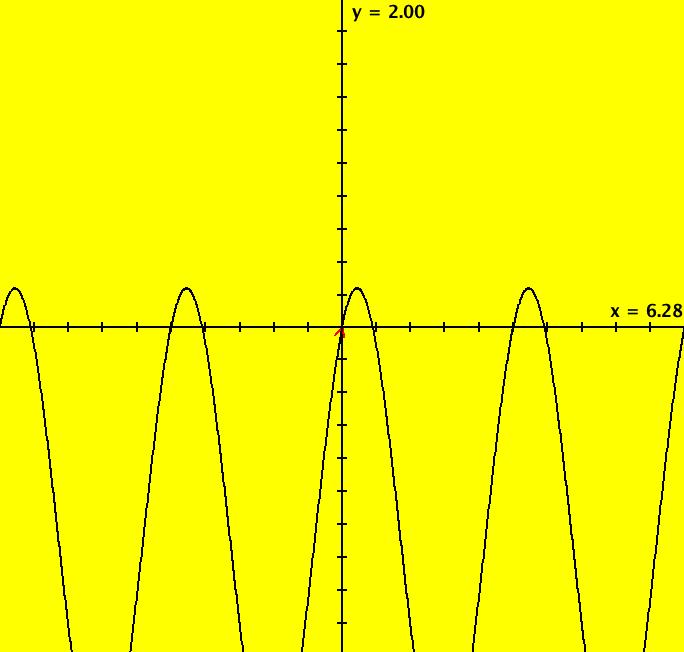
View/Sys/Gal: Ode "Ex 1b: y = abs(a*sin(b*x+c)), a=1; b=1; c=0 on x ∈ [-π,π]" in "PlottingCurves." Case 1: y = f(x), f smooth or not, with or without parameters. This ode is defined by the equation: dx/dt = abs(a*sin(b*x+c)) in the (t,x) coordinate system. Parameters are: a=1; b=1; c=0 The red curve is "y = abs(a*sin(b*x+c))" rotated π/2 ccw. Image 1: y = abs(a*sin(b*x+c)), a=1; b=1; c=0 Vary a, b and/or c.
|
|
|
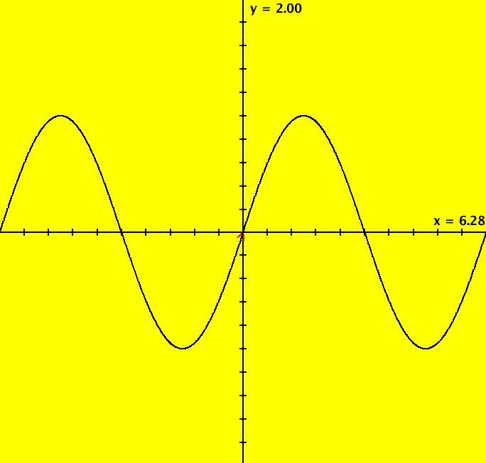
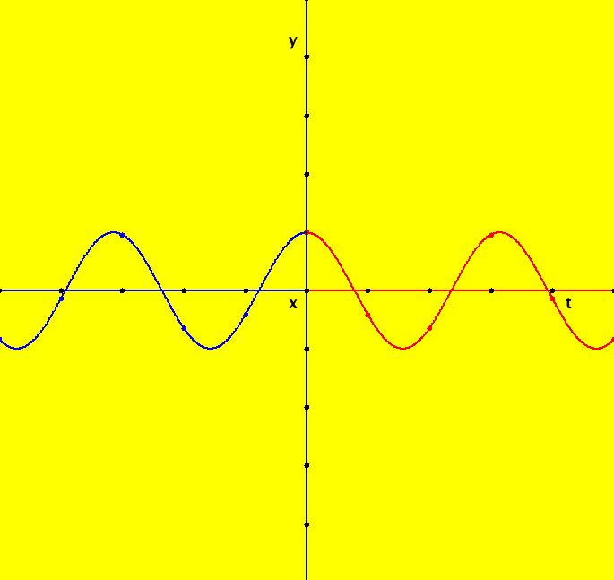
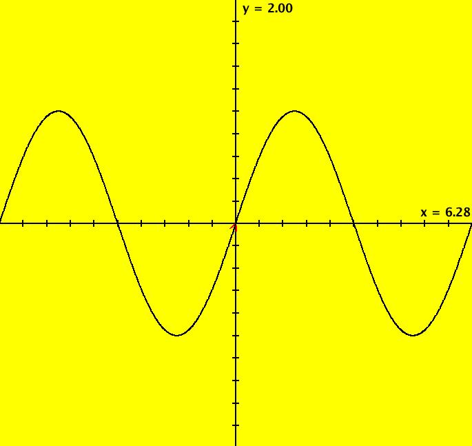
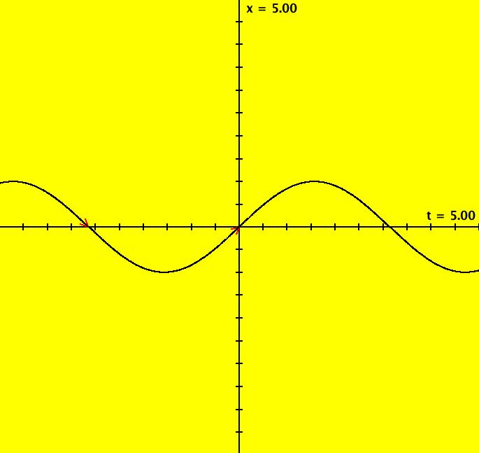
View/Sys/Gal: Ode "Ex 2: y = sin(x) on x ∈ [-π,π]" in "PlottingCurves." Case 2: y = f(x), f smooth, no parameters. Plot y = sin(x) on x ∈ [- π, π]. The system of odes is defined by the equations: dx/dt = 1, dy/dt = df/dx = cos(x), ICs: (0,0) are on y = sin(x). Image 1: y = sin(x) on x ∈ [- π, π]. Using other ICs gives y = sin(x) translated in the y direction. Image 2: y = sin(x)+y(0), ICs: (2.340517,-0.420202)
|
|
|
View/Sys/Gal: Ode "Ex 2b: y = a*sin(b*x+c), a=1; b=1; c=0" in "PlottingCurves." Case 2: y = f(x), f smooth but w/parameters. Plot y = a*sin(b*x+c). This system of odes is defined by the equations: dx/dt = 1, dy/dt = a*cos(b*x+c)*b. Parameters are: a=1; b=1; c=0 ICs: (0,0). Parameter "a" adjusts the amplitude, b adjusts the frequency and c translates the curve. If you adjust a and/or b the curve is a sin curve about the x axis but if you adjust c it is no longer a sin curve about the x axis. Image 1: y ≠ a*sin(b*x+c), a=1.5; b=2; c=1 Image 2: y = a*sin(b*x+c), a=1; b=1; c=0
|
|
|
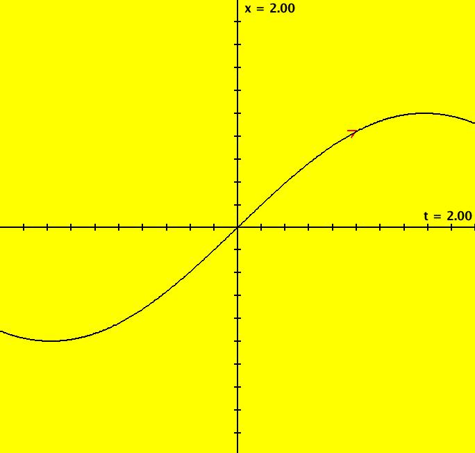
View/Sys/Gal: Ode "Ex 2c: plot sin(t) and integrate cos(t) on [1,2]" in "PlottingCurves." Case 2b: x = f(t), integrate f'. This ode is defined by the equation: dx/dt = cos(t) in the (t,x) coordinate system. ICs: (1,sin(1)) = (1,.84147099) With hMax = 2 and the Bdr closed, x(2) = 0.9092974268259170 so the integral of cos(t) on [1,2] is, using OdeFactory, 0.9092974268259170-0.8414709848078965 = 0.06782644201 802 The exact answer is sin(2) - sin(1) = 0.06782644201 77852 WA gives integral of cos(t) on [1,2] = 0.06782644201 77852 Image 1: sin(t) on [-2,2], ICs: (1,sin(1)), w/Bdr closed.
|
|
|
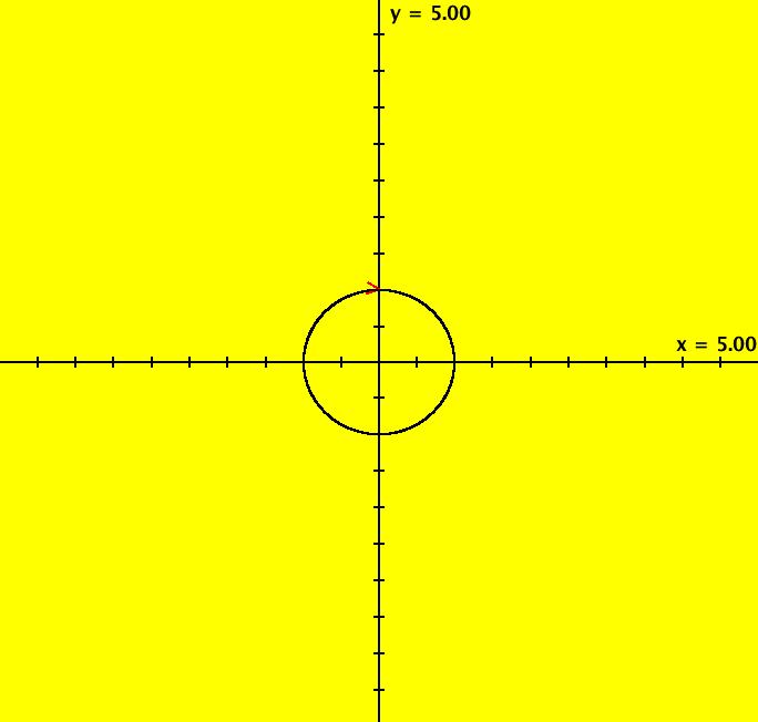
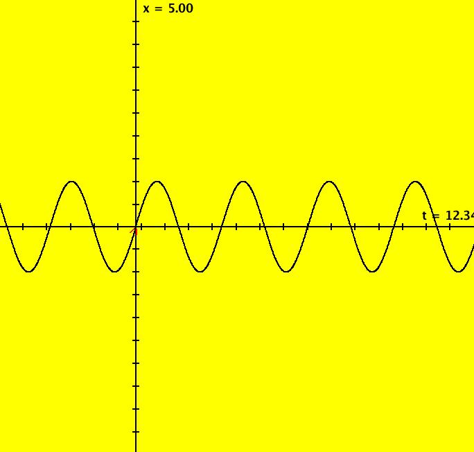
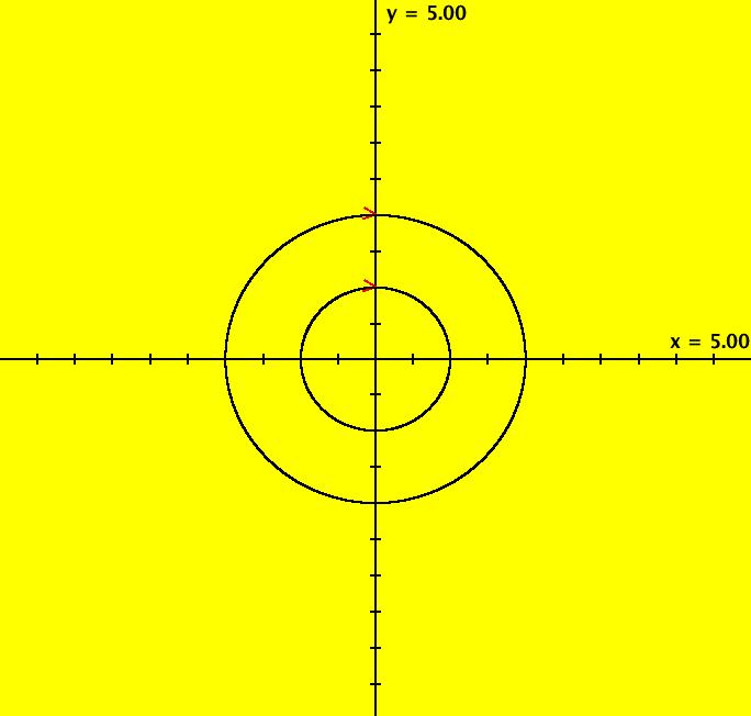
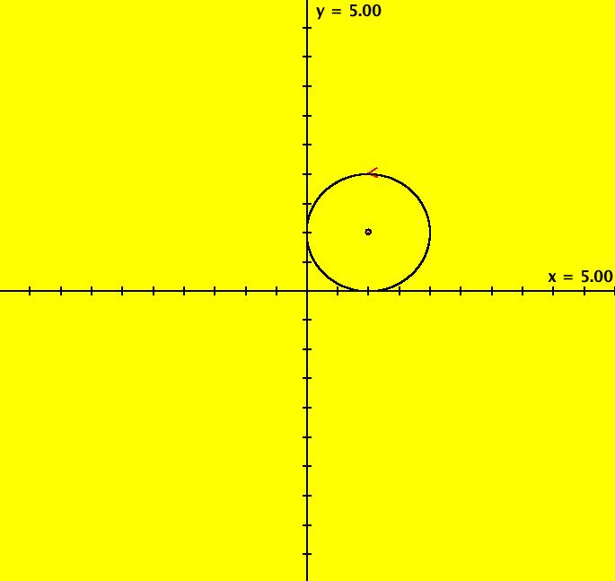
View/Sys/Gal: EMap "Ex 3: H(x,y) = x^2+y^2 = 1" in "PlottingCurves." Case 3: H(x,y) = c, H smooth. H = x^2+y^2 = 1, circle of r = 1. This system of odes is defined by the equations: dx/dt = 2*y, dy/dt = -2*x. ICs: (x,y) = (0,1). This is the unit circle about the origin. Image 1: The unit circle centered at the origin. As a check of RK4, the computed values of x(100) and y(100) are: p(100.000000) = (-0.873297,0.487187) The closed form solution is: x(t) = sin(2*t), y(t) = cos(2*t) which gives: x(100) = sin(200) = -0.8732972 y(100) = cos(200) = 0.4871876 If you center at (0,1) and zoom in 7X you can see that the computed trajectory spiral in. Image 2: Centered at (0,1), zoomed in 7X. To see x(t) and y(t) enter the 3D view then select the 3D/(t,x) and 3D/(t,y) views. Image 3: x(t) in the 3D/(t,x) view. Find x(12.345) using OdeFactory by starting a solution in the (t,x) view at (t,x,y) = (0,0,1). Set hMax = 12.345, close the border, click on the arrowhead and read p(12.345000) = (-0.428418,0.903581) Image 4: x(t) defined in the (t,x) view. So OdeFactory gives x(12.345) = -0.428418. The exact value of x(12.345) = sin(2*12.345) = -.42841478. Image 5: ICs: (0,2) gives a circle of radius 2. Image 6: EMapCT9 view.
|
|
|
View/Sys/Gal: Ode "Ex 3b: ((a*(2*y)),-(a*(2*x))), a = 1; , H=x^2+y^2" in "PlottingCurves." Case 3: H(x,y) = c, H smooth. Only H = x^2+y^2 was entered in the "user fns:" field. OdeFactory created the system. This system of odes is defined by the equations: dx/dt = (a*(2*y)), dy/dt = -(a*(2*x)). Parameters are: a = 1; Functions are: H=x^2+y^2 ICs: (0,1). Image 1: H=x^2+y^2=1 Image 2: 3D/(t,x) shows x(t) = sin(t). Image 3: 3D/(t,y) shows y(t) = cos(t). Image 4: 3D/(t,x,y) view. The solution curve on the unit cylinder. (x(t),y(t)) is the parametric representation of the circle x^2+y^2 = 1.
|
|
|
View/Sys/Gal: Ode "Ex 3c: H=(x-a)^2+(y-b)^2, ((c*(2*y-2*b)),-(c*(2*x-2a))), a=1; b=1; c = 1;" in "PlottingCurves." Case 3: H(x,y) = c, H smooth. Circles centered at (a,b) = (1,1). Only H = (x-a)^2+(y-b)^2, a=1 and b=1 were entered. OdeFactory created the system. This system of odes is defined by the equations: dx/dt = (c*(2*y-2*b)), dy/dt = -(c*(2*x-2*a)). Parameters are: a=1; b=1; c = 1; Functions are: H=(x-a)^2+(y-b)^2 ICs: (1,2). Circle centered at (a,b) = (1,2). The ICs determine r. The parameter c is created by OdeFactory when it generates the system. Parameter c determines the rate and direction of the motion. Image 1: c = -1, ccw rotation Image 2: c = 0, no rotation, no circle, dx/dt = dy/dt = 0 Image 3: c = 1, cw rotation
|
|
|
View/Sys/Gal: Ode "Ex 3d: H=y-sin(x), ((a),-(a*(-1*cos(x)))), a = 1;" in "PlottingCurves." Case 3: H(x,y) = c, H smooth. Plot y = sin(x) on x ∈ [- π, π]. This is really a case 2 example done as a case 3 example (i.e. case 2 is a special case of case 3). Create the system by entering H = y-sin(x) in the "user fns:" field and let OdeFactory generate the system. The system of odes is defined by the equations: dx/dt = (a), dy/dt = -(a*(-1*cos(x))). Parameters are: a = 1; The parameter "a" is generated by OdeFactory. If case 3 is implemented by hand you get: dx/dt = 1, dy/dt = -cos(x). Functions are: H=y-sin(x) ICs: (0,0) is on the curve H = 0, i.e. on y = sin(x). If you use different ICs you get translates of y = sin(x) in the y direction. Image 1: y = sin(x) starting from H=y-sin(x).
|
|
|
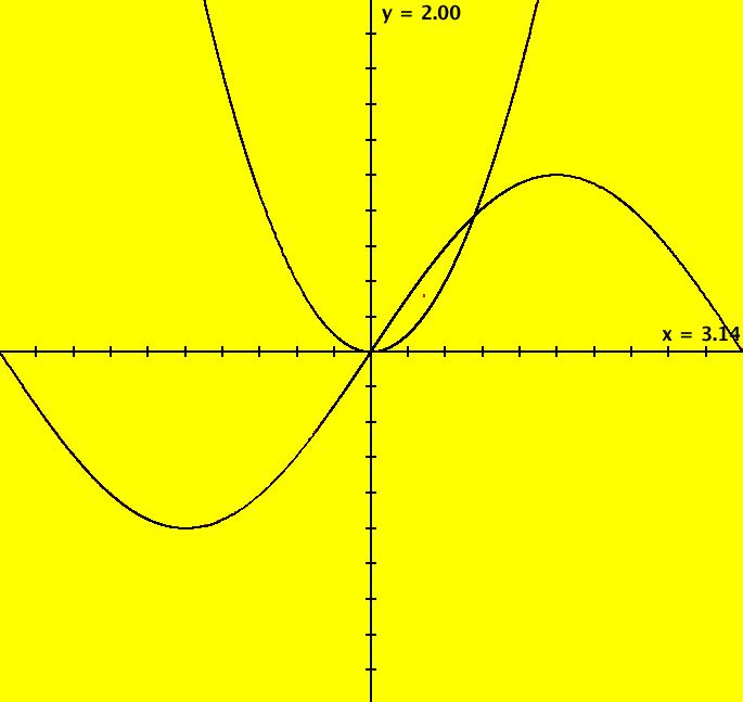
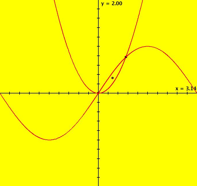
View/Sys/Gal: Ode "Ex 3e: H=y-sin(x); P=y-x^2, plotting two curves" in "PlottingCurves." This is a quasiHamiltonian system. It is a Hamiltonian system iff a = b. H and P are the generating curves. Segments of H and P, that contain ICs on H and P, are on trajectories but H and P are not themselves trajectories. Trajectories with ICs not on H or P are not sin curves or parabolas. H and P form the separatrix system. This system of odes is defined by the equations: dx/dt = (a*P+b*H), dy/dt = -(a*(-1*cos(x))*P+b*(-2*x)*H). Parameters are: a = 1; b = 1; Functions are: H=y-sin(x); P=y-x^2 ICs: (+-1,1), (.5,.25) on P, ~(0,0), ~(.876,.768) on H and P, ~(0.450951,0.320000) 3rd fixed point. Image 1: A sin curve and a parabola with "Hide Arrowheads/Seeds" off. Image 2: Black trajectories deleted, red trajectories are separatrices. The separatrices were created first. To create a separatrix: - turn the colored vector field on, - zoom in on a nullcline crossing, - start trajs on edge of black region. Image 3: The R2+ view showing the (red) separatrix system and the global phase portrait of the system.
|
|
|
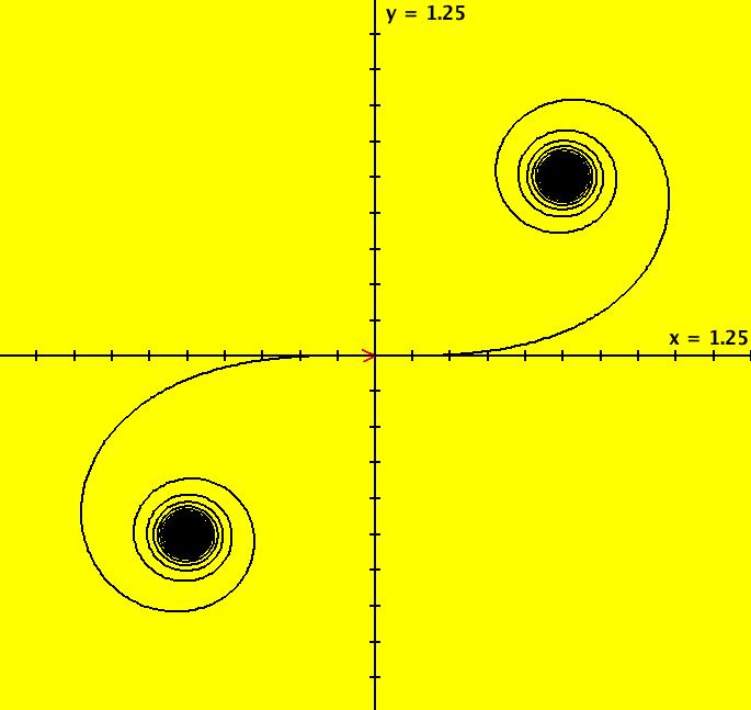
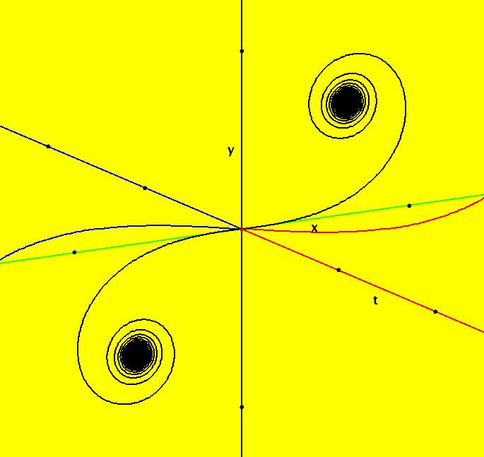
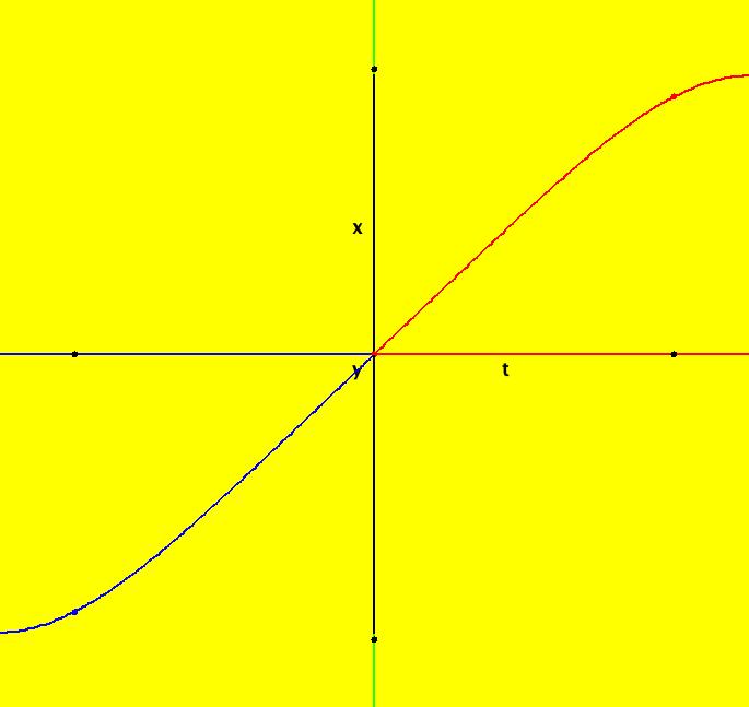
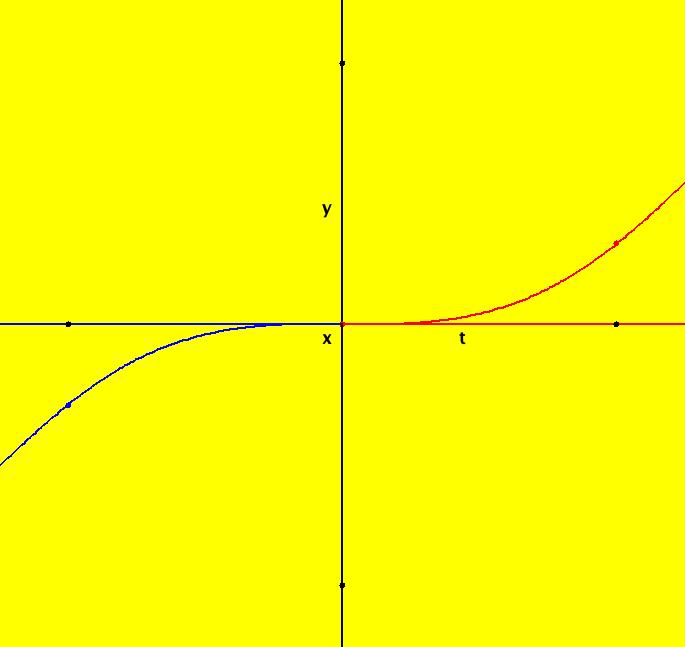
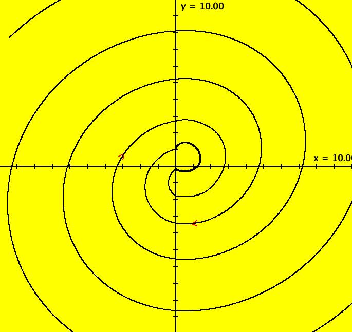
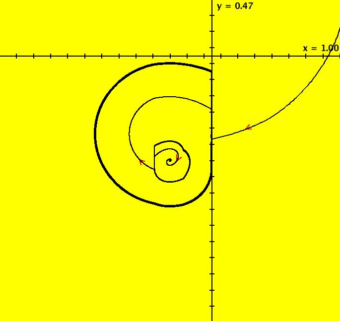
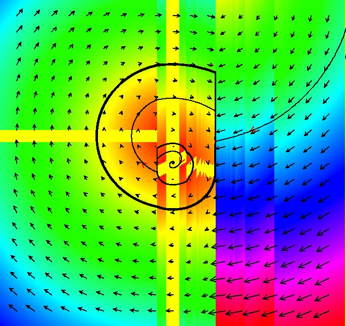
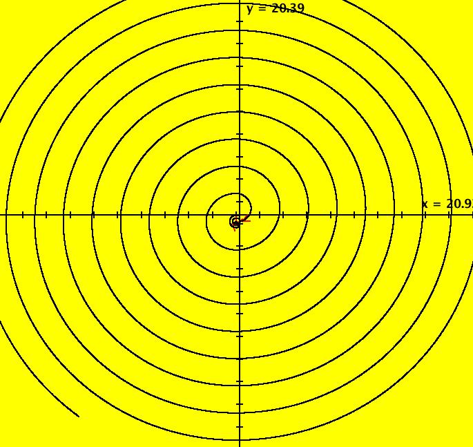
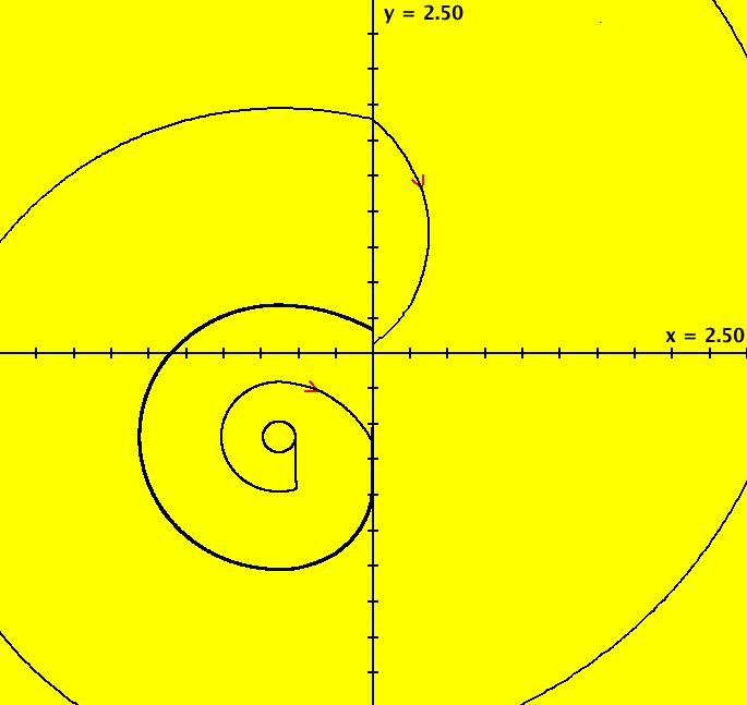
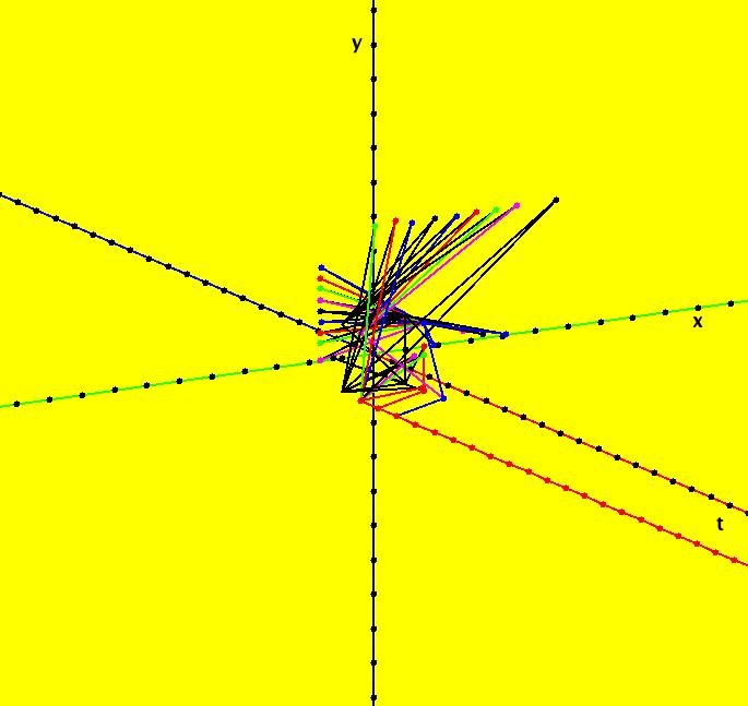
View/Sys/Gal: Ode "Ex 4: Fresnel C(t) and S(t) functions and the Euler spiral" in "PlottingCurves." Plot the Fresnel C(t) and S(t) functions defined by: C(t) = ∫ cos(t^2), S(t) = ∫ sin(t^2). Use the nonautonomous non-coupled system of odes defined by the equations: dx/dt = cos(t^2), dy/dt = sin(t^2), w/ICs (0,0). Note that in OdeFactory x(t) is C(t) and y(t) is S(t). One way to see C(t) and S(t) is to use 3D/(t,x) and 3D/(t,y). In the (x,y) view we have the Euler spiral, also known as Cornu spiral or clothoid. It is the curve generated by a parametric plot of (x(t),y(t)), i.e. (C(t),S(t)). The the spirals are centered at: +-(sqrt( π/8),sqrt( π/8)). If (x(0),y(0)) is not (0,0) you get a translated version of the Euler spiral. Image 1: Euler spiral. Image 2: Euler spiral, 3D/(t,x,y) view of image 1 zoomed out 2X. Image 3: Euler spiral, 3D/(t,x) view of image 1 zoomed out 2X shows C(t). Image 4: Euler spiral, 3D/(t,y) view of image 1 zoomed out 2X shows S(t). Another way to plot C(t) and S(t) is to start trajectories at (0,0,0) in the (t,x) and (t,y) views. Image 5: C(t) in the (t,x) view. Image 6: S(t) in the (t,y) view. See Fresnel functions.
|
|
An OdeFactory Slide Show Click on a slide to zoom in. Click "video" to see a video. |
View/Sys/Gal: Ode "Ex 5: plot C(t) and S(t) using WA" in "PlottingCurves." Open WA from the Help menu then copy/paste the following line into WA: plot (C(x),S(x)) Also try WA on: plot y = abs(a*sin(b*x+c)) for a=1, b=1, c=0 Vary a, b and/or c by entering different values in WA.
|
|
An OdeFactory Slide Show Click on a slide to zoom in. Click "video" to see a video. |
View/Sys/Gal: Ode "MoreExs: Simpson's Rule & RK4" in "PlottingCurves." ~~~~~~~~~~ Simpson's Rule & RK4 ~~~~~~~~~~~~ A method of plotting a function f(t), which is based on the fundamental theorem of calculus, works for differentiable functions. It plots the function f(t) and enables you to find the definite integral of the function f'(t) on the interval [a,b]. To plot the function f(t) define the nonautonomous 1D system dx/dt = f'(t). Use ICs on the f(t) curve. Here is why the method works. If x(t) is differentiable and I is the integral operator and D is the derivative operator, then the Fundamental Theorem of Calculus says that integration and differentiation are inverse operators to within a constant, that is, I(D(x(t)))- D(I(x(t))) = c The constant c has to do with the differential equation's initial conditions. Symbolically, if dx/dt = f(t) (1) with ICs on f(t) then dx = f(t)dt and ∫ dx = ∫ f(t)dt or x(t) = ∫ f(t)dt (2) When you apply OdeFactory to (1) and use ICs on f(t), RK4 computes and plots the curve x(t) in +-t. When the integral in (2) can be found as a finite algebraic expression involving elementary functions, x(t) is said to be a "closed" form solution to the ode. As early as 1775 mathematicians realized that finding closed form solutions to most odes is not possible. Hint: if you need a closed form solution to prove a general property of x(t) or to find the most accurate value of x(t), you can use WolframAlpha, or Mathematica, to find it - if a closed form solution exists. Applying Simpson's rule to (2) also produces the solution curve x(t) since, for 1D autonomous odes, RK4 is equivalent to Simpson's rule. It is important to note that all odes define functions but that only a few "elementary" functions have names and are implemented with fast algorithms, as "built-in" functions, in programming languages. You can think of RK4 as a machine that transforms input functions into output functions: input = algebraic fns --> RK4 --> output = algebraic fns + other fns Some of the "other fns" have names but they are defined, and computed, as integrals using numerical integration methods. See the Fresnel S function for example. See special functions.
|
|
|
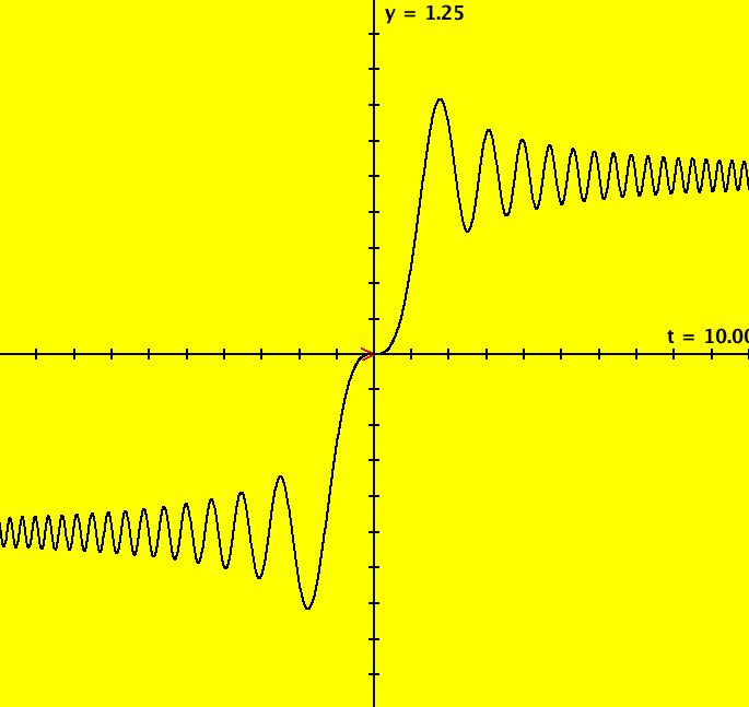
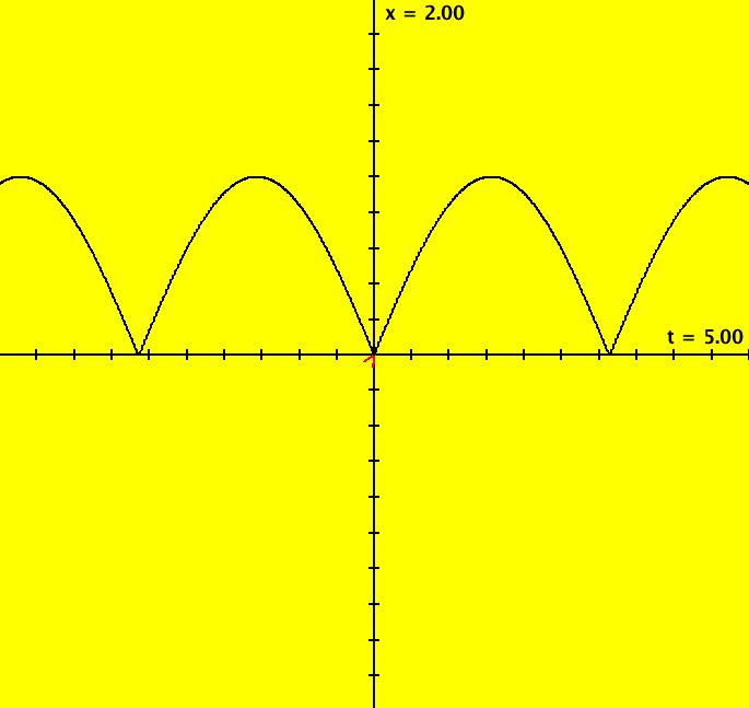
View/Sys/Gal: Ode "MoreExs: plot x(t) = abs(sin(t)) using dx/dt = cos(t)*sgn(sin(t)) w/ICs (0,0) " in "PlottingCurves." This ode is defined by the equation: dx/dt = cos(t)*sgn(sin(t)) in the (t,x) coordinate system. To plot x(t) = abs(sin(t)) = f(t) use dx/dt = df/dt. f(t) is not really differentiable at multiples of π. However x(t) = sin(t) if sin(t) >= 0 and x(t) = -sin(t) if sin(t) < 0 so df/dt = cos(t) if sin(t) >= 0 and df/dt = -cos(t) if sin(t) < 0 so dx/dt = cos(t)*sgn(sin(t). Image 1: x(t) = abs(sin(t)).
|
|
|
View/Sys/Gal: Ode "MoreExs: plot x(t) = abs(t) using dx/dt = abs(x)" in "PlottingCurves." This ode is defined by the equation: dx/dt = abs(x) in the (t,x) coordinate system. Image 1: The red curve is y = abs(x) rotated 90 degrees ccw.
|
|
|
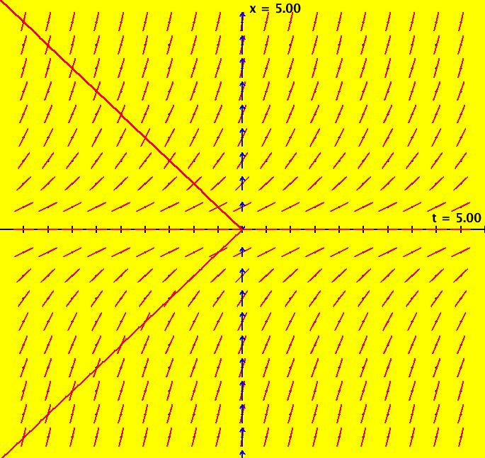
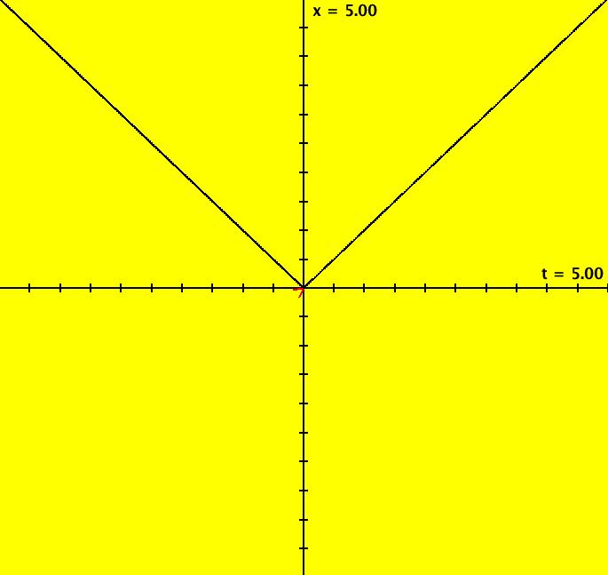
View/Sys/Gal: Ode "MoreExs: plot x(t) = abs(t) using dx/dt = sgn(t), w/ICs (0,0)" in "PlottingCurves." df/dt does not exist at t = 0 but we can plot x(t) = abs(t) = f(t) using dx/dt = df/dt = sgn(t), w/ICs x(0) = 0. Image 1: x(t) = abs(t).
|
|
|
View/Sys/Gal: Ode "MoreExs: plot x(t) = cos(t) using dx/dt = -sin(t), w/ICs (0,1)" in "PlottingCurves." Plot x(t) = cos(t) using dx/dt = -sin(t), w/ICs x(0) = 1. Image 1: x(t) = cos(t)
|
|
|
View/Sys/Gal: Ode "MoreExs: plot x(t) = sin(t) using dx/dt = cos(t), w/ICs (0,0) and integrate cos(t) on [-5,5]" in "PlottingCurves." The goal here is to plot the function f(t) = sin(t) by using f'(t) and to find the integral of f'(t) on [a,b]. This ode is defined by the equation: dx/dt = df/dt = cos(t) (1) in the (t,x) coordinate system. To "solve" the ode, using calculus, means to find a function x(t) that makes (1) true. To find x(t) integrate both sides of (1) with respect to t to get ∫ dx/dt dt = ∫ cos(t) dt or ∫ dx = x+c1 = sin(t)+c2 so x(t) = sin(t)+c. (2) x(t) is a family of curves in the extended phase space, (t,x). We see that each x(t) is just the sin(t) curve shifted up if c > 0 or down if c < 0. Starting a solution at any point (t*,sin(t*)) on the sin(t) curve gives x(t*) = sin(t*)+c, but x(t*) = sin(t*) so sin(t*) = sin(t*)+c and c = 0. ICs: (0,0), (- π,0) define two solution curves that lie on top of each other. To see that the two solution curves are just phase shifted versions of each other start a Flow. To find the "integral" of cos(t) on [-5,5], close the border then click on either arrowhead to get: p(5.0000000000000000) = (-0.9589242746665082) p(0.0000000000000000) = (0.0000000000000000) p(-5.0000000000000000) = (0.9589242746665082) So the integral of cos(t) on [-5,5] is x(5)-x(-5) = (-0.9589242746665082)-0.9589242746665082) = -1.9178 4854 9333 0164 Applying WA to integral of cos(t) on [-5,5] gives -1.9178 4854 9326 28 In summary: - to plot f(t), solve dx/dt = f'(t) with ICs p = (t,f(t)). - to integrate f'(t) on [a,b] = [hMin,hMax], solve dx/dt = f'(t) with ICs p = (t,f(t)), close the border, click on p then compute p(b)-p(a). Image 1: x(t) = sin(t) on t ∈ [-5,5]
|
|
|
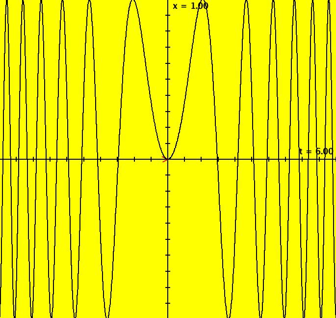
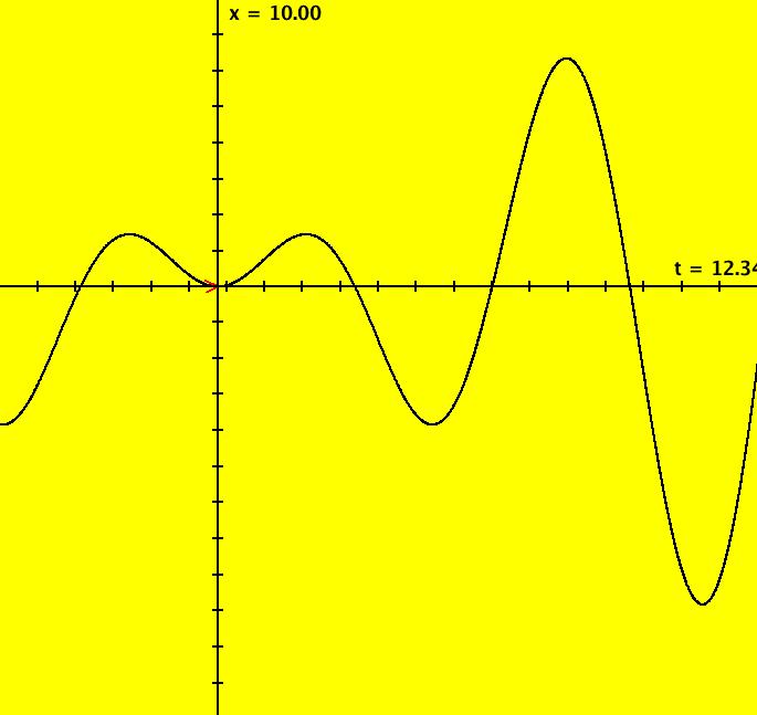
View/Sys/Gal: Ode "MoreExs: plot x(t) = sin(t^2) using dx/dt = cos(t^2)*2*t" in "PlottingCurves." This ode is defined by the equation: dx/dt = cos(t^2)*2*t in the (t,x) coordinate system. The curve is x(t) = sin(t^2). The integral from 0 to b > 0 of sin(t^2) stays > 0 because a positive hump always has more area under it than the next negative hump. Image 1: x(t) = sin(t^2) on t ∈ [-6,6] Apply WA to x(t) = sin(t^2)
|
|
|
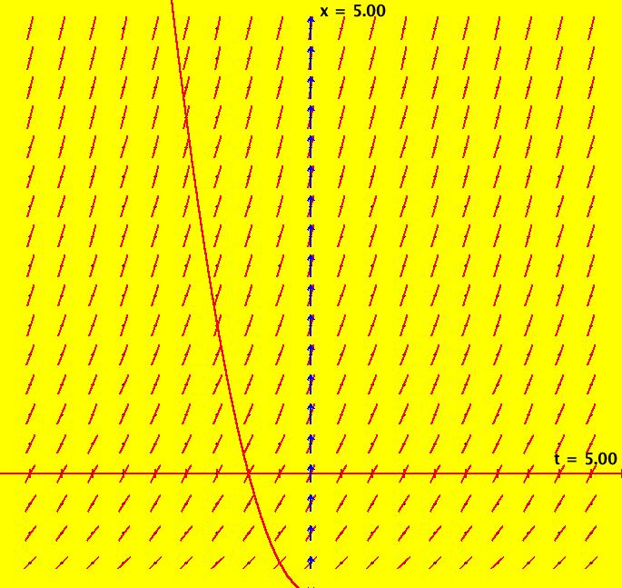
View/Sys/Gal: Ode "MoreExs: plot x(t) = sin(t^2) using dx/dt = sin(x^2) w/slope fld on" in "PlottingCurves." This ode is defined by the equation: dx/dt = sin(x^2) in the (t,x) coordinate system. Image 1: y = sin(x^2).
|
|
|
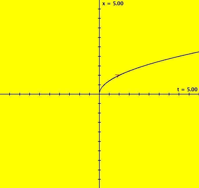
View/Sys/Gal: Ode "MoreExs: plot x(t) = sqrt(t), t > 0 using dx/dt = .5/sqrt(t), w/ICs (1,1)" in "PlottingCurves." Plot x(t) = sqrt(t), t > 0 using dx/dt = .5/sqrt(t), w/ICs x(1) = 1. Image 1: x(t) = sqrt(t). If you try using ICs (-1,1) OdeFactory gives you an error message.
|
|
|
View/Sys/Gal: Ode "MoreExs: plot x(t) = sqrt(t), t > 0 using dx/dt = sqrt(x) w/slope on" in "PlottingCurves." This ode is defined by the equation: dx/dt = sqrt(x) for x >= 0 in the (t,x) coordinate system. Image 1: y = sqrt(x), x >= 0
|
|
|
View/Sys/Gal: Ode "MoreExs: plot x(t) = t*sin(t) using dx/dt = sin(t)+t*cos(t) and find x(12.24)" in "PlottingCurves." To find the value of f(t) = t*sin(t) at t = 12.34 let dx/dt = f'(t) = sin(t)+t*cos(t). Set ICs x(0) = 0 and hMax = 12.34. Close the border and set vMax and vMin so that vMin < x(t) < vMax. Click on the arrowhead to get p(12.340000) = (-2.769617). The exact answer is -2.7696209. Image 1: x(t) = t*sin(t) on t ∈ [-5,12.34]
|
|
|
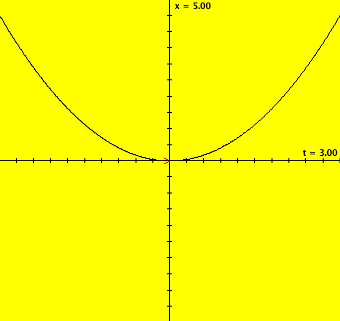
View/Sys/Gal: Ode "MoreExs: plot x(t) = t^2/2 using dx/dt = t, w/ICs {0,0} and integrate t on [0,3]" in "PlottingCurves." This ode is defined by the equation: dx/dt = t in the (t,x) coordinate system. ICs: (t,x) = (0,0). The closed form solution is: x(t) = t^2/2+x(0). Image 1: x(t) = t^2/2 on t ∈ [-3,3] To find the "integral" of f(t) = t on [0,3], click on the arrowhead to get: p(3.000000) = (4.500000) p(0.000000) = (0.000000) p(-3.000000) = (4.500000) So the integral is x(3)-x(0) = 4.500000-0 = 4.5
|
|
|
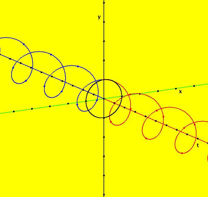
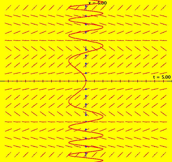
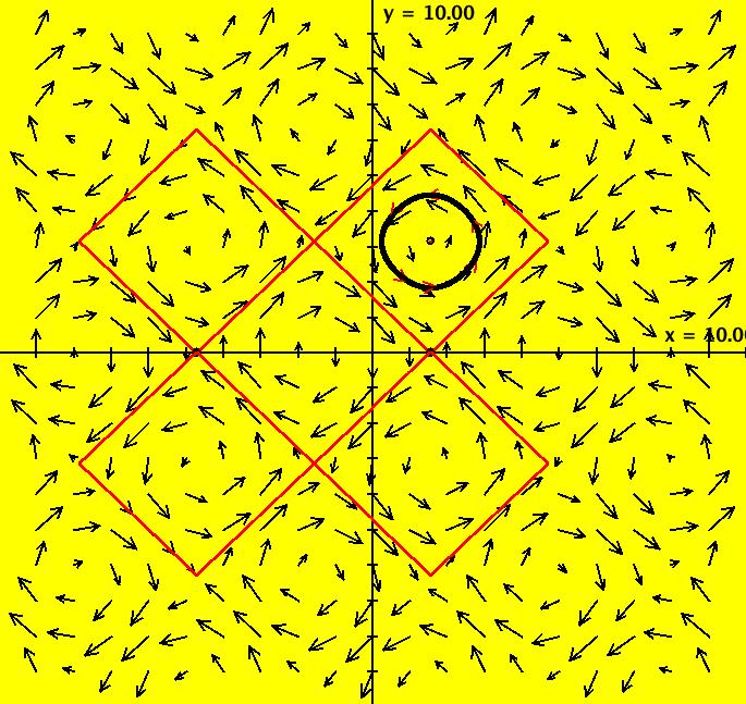
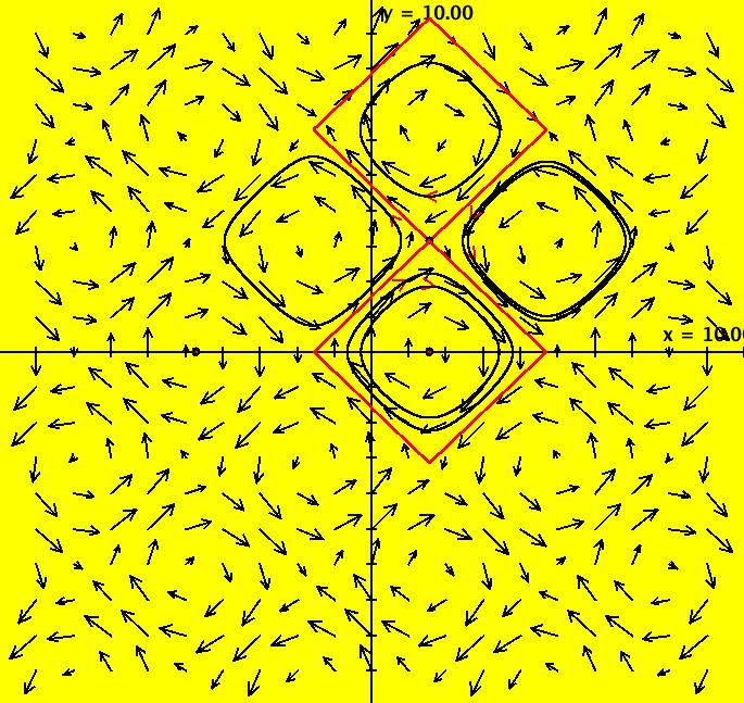
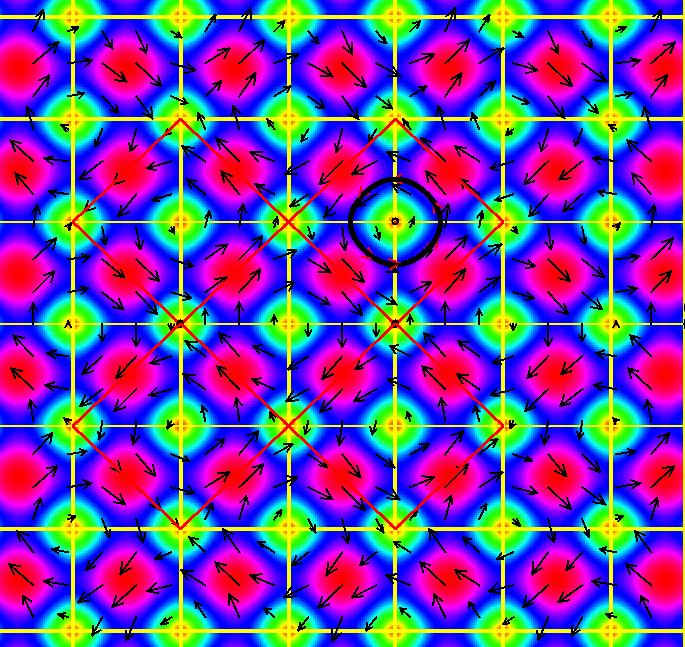
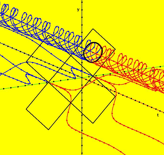
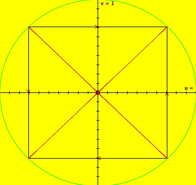
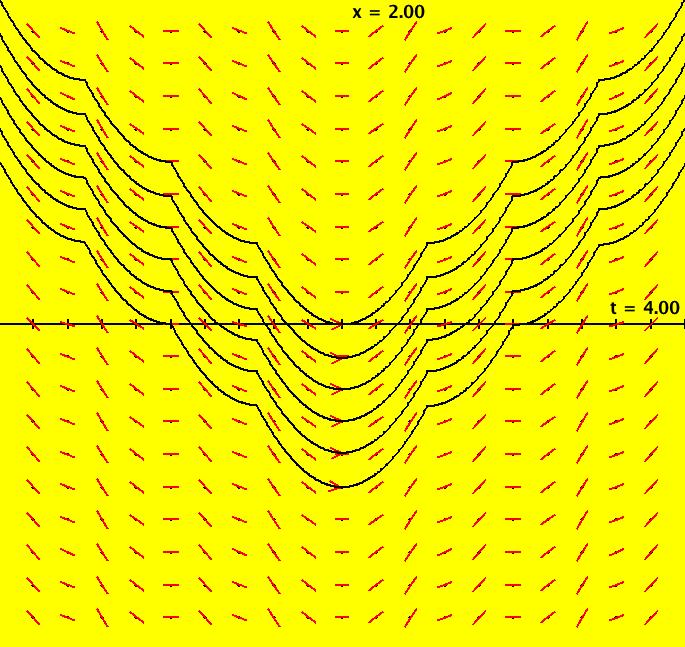
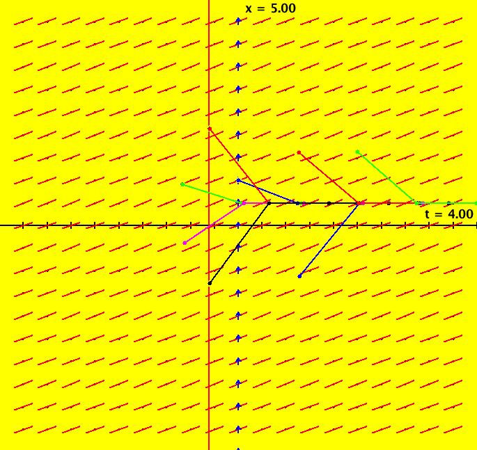
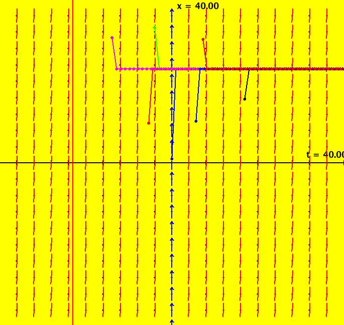
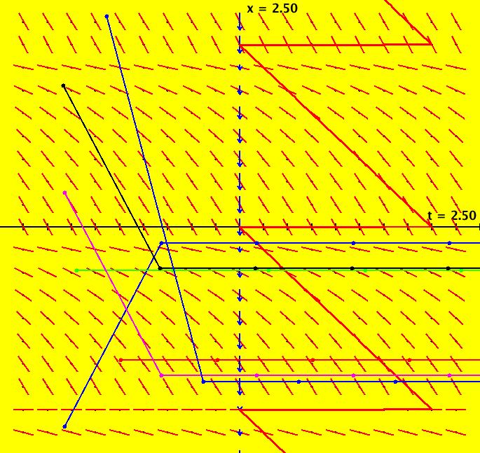
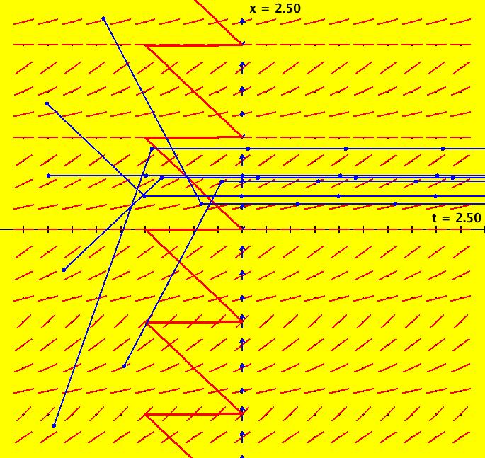
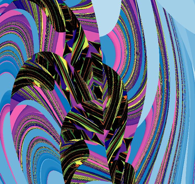
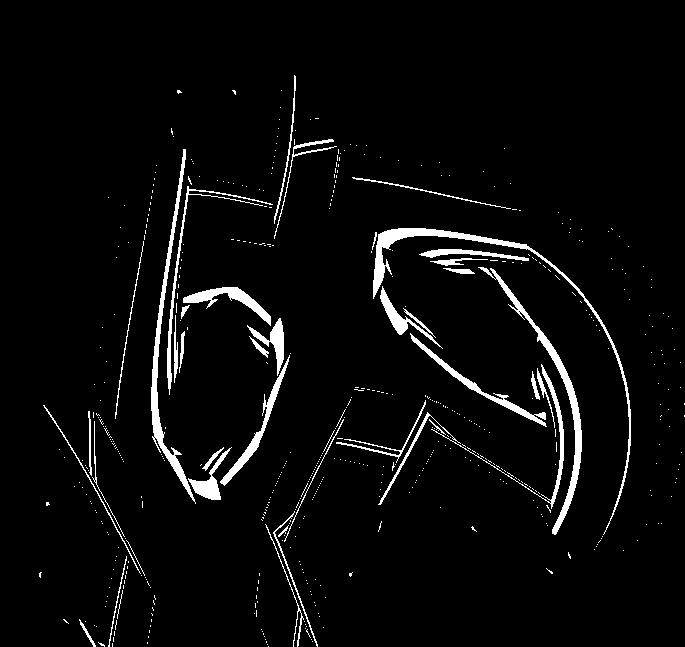
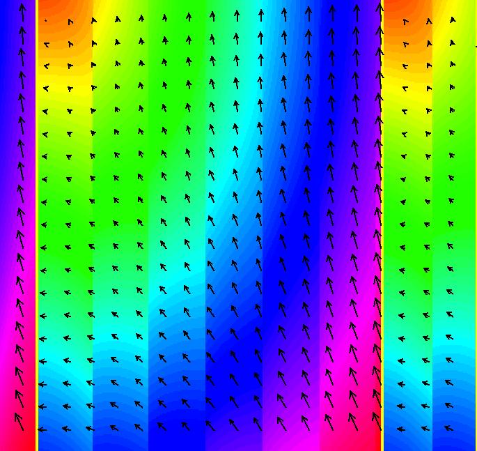
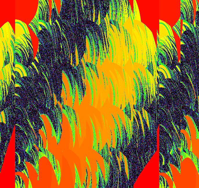
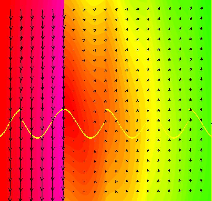
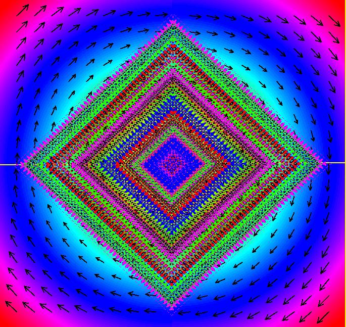
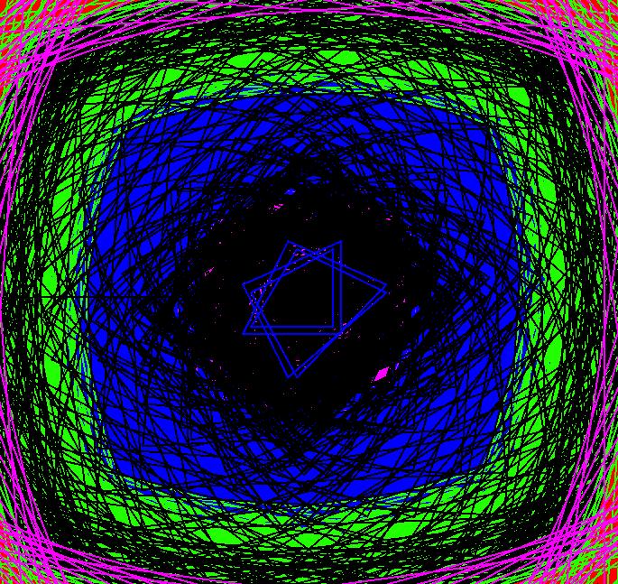
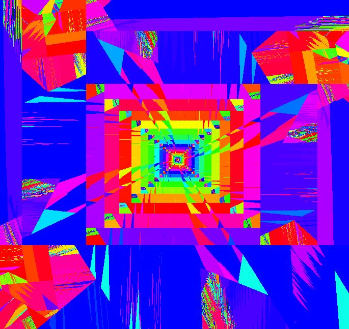
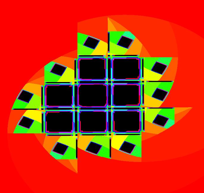
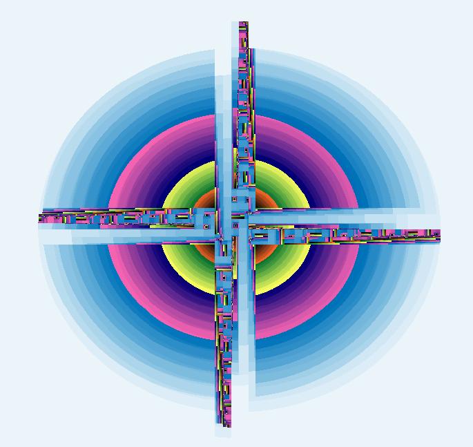
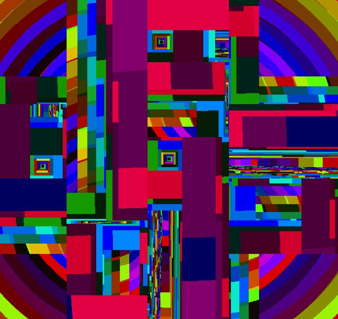
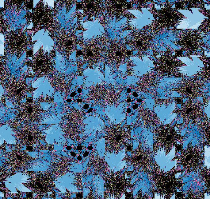
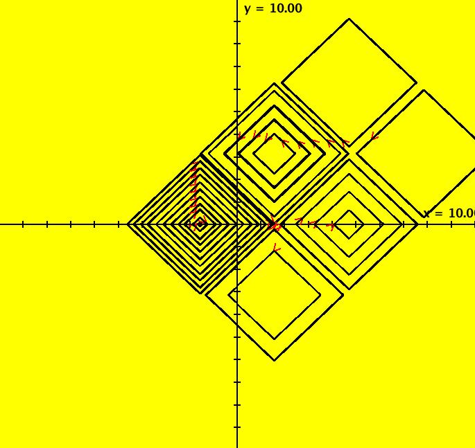
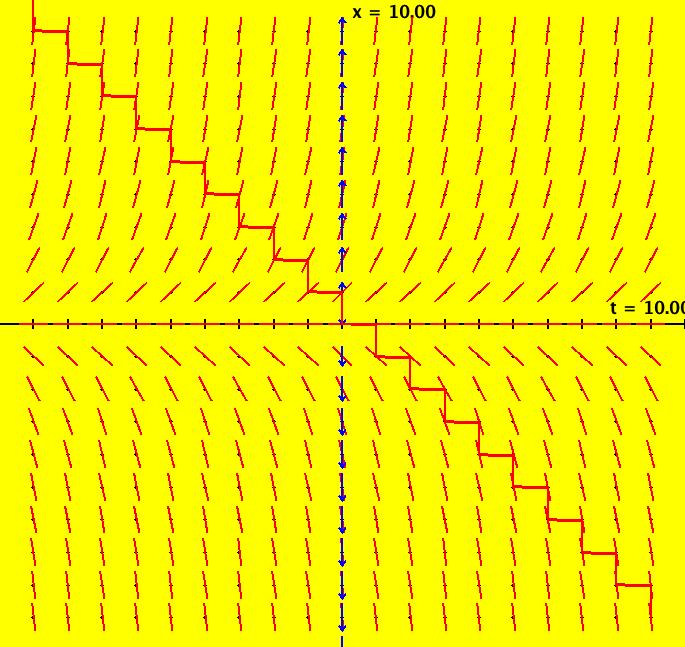
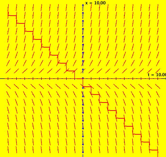
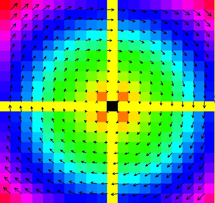
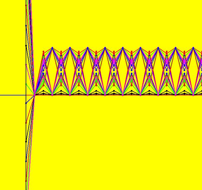
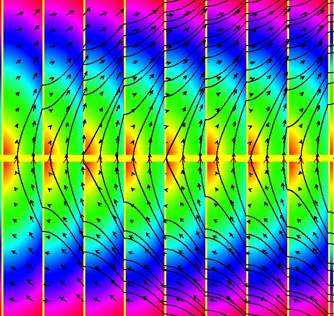
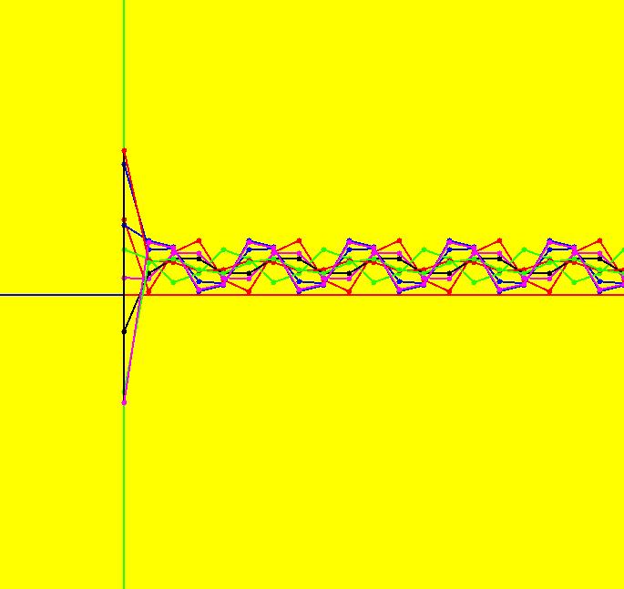
View/Sys/Gal: Ode "MoreExs: plot x(t) = ∫sin(y), y(t) = ∫a*cos(x), a = -1.00; " in "PlottingCurves." Plot the family of nameless curves defined by the integrals: x(t) = ∫ sin(y(t)) dt, y(t) = ∫ a*cos(x(t)) dt. This system of odes is defined by the equations: dx/dt = sin(y), dy/dt = a*cos(x). Parameters are: a = -1.00; For a = -1: the red squares are form the (infinite) separatrix system. There is a fixed point at the center of each red square (see the upper right red square). For a = 1: the corners of the red squares become fixed points and the old fixed points become corners of the new separatrix system. Image 1: a = -1, Ode view w/vector field on. Image 2: a = 1, Ode view w/vector field on. Image 3: a = -1, Ode view w/colored vector field on. Image 4: a = -1, Ode 3D/(t,x,y) view.
|
|
|
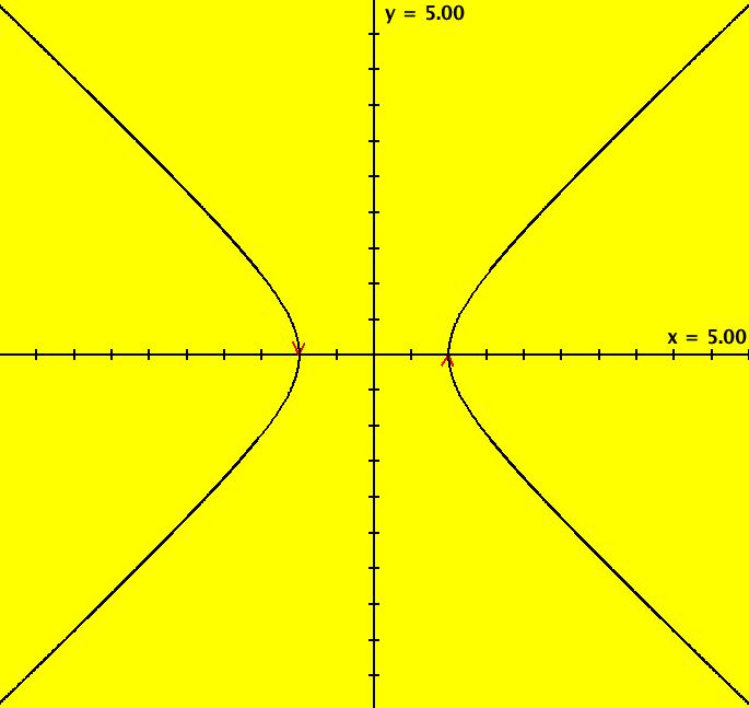
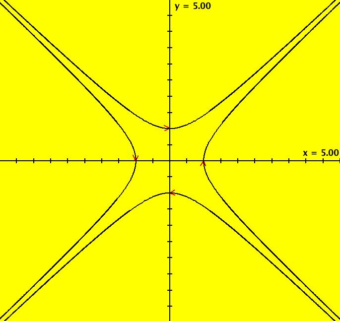
View/Sys/Gal: Ode "MoreExs: plot x^2-y^2=1 using dx/dt = 2*y, dy/dt = 2*x" in "PlottingCurves." This system of odes is defined by the equations: dx/dt = 2*y, dy/dt = 2*x. The desired curve is given by x^2-y^2 = 1. Let H = 1-x*2+y^2 and define the Hamiltonian system dx/dt = ∂H/ ∂y = 2*y, dy/dt = - ∂H/ ∂x = 2^x and use ICs on H = 0: (1,0), (-1,0) to generate the two branches of the curve. Image 1: The hyperbola x^2-y^2 = 1. Image 2: ICs (0,1), (0,-1) give the hyperbola x^2-y^2 = -1. Image 3: The R2+ view with separatrices added.
|
|
An OdeFactory Slide Show Click on a slide to zoom in. Click "video" to see a video. |
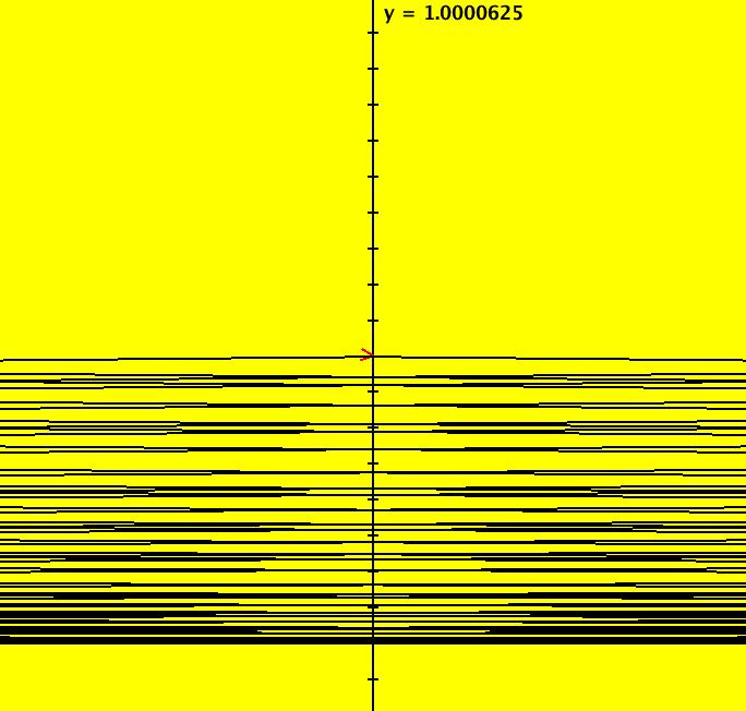
View/Sys/Gal: Ode "NonSmoothExs: Plotting Nonsmooth Functions" in "PlottingCurves." Nonsmooth functions can be used in OdeFactory to create interesting generative art,or "GenArt" for short, using the IMap or EMap views. The following systems show how to define, plot and use nonsmooth functions. Most of the previous systems demonstrated how to use OdeFactory to plot smooth functions and 2D curves. The basic idea was to plot x = f(t) by using OdeFactory to plot the solution to dx/dt = f'(t) w/ICs x(0) = f(0). In the case of smooth 2D curves, a Hamiltonian system was used. When f' does not exist at some points in the domain of interest, the "dx/dt = f'(t)" method generally cannot be used. However, it is still easy to see what "f(t)" looks like by defining the companion system dx/dt = f(x) and viewing the system with the slope field on. The function f(x) is drawn in red about the x axis and the f(x) curve, when rotated 90 degrees clockwise, is "y = f(x)."
|
|
|
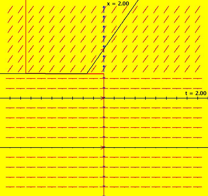
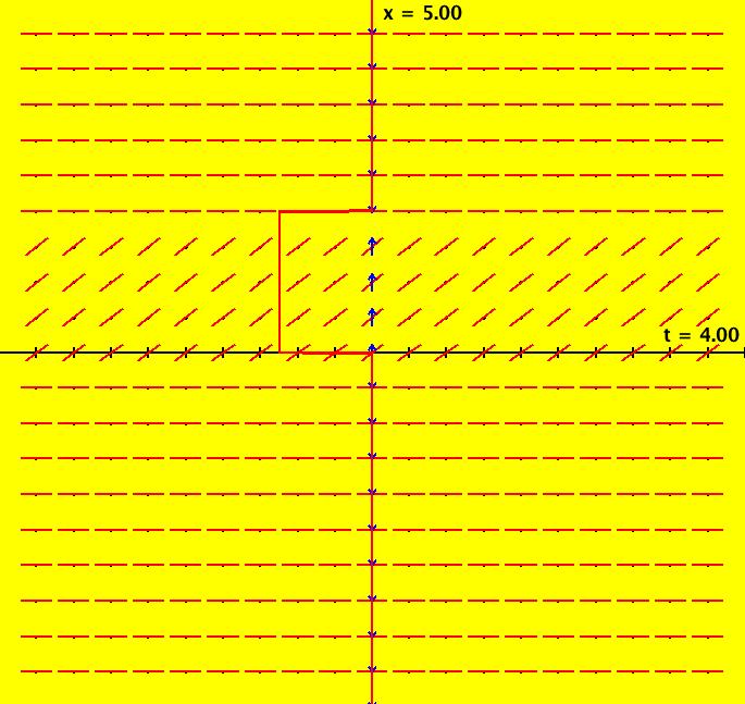
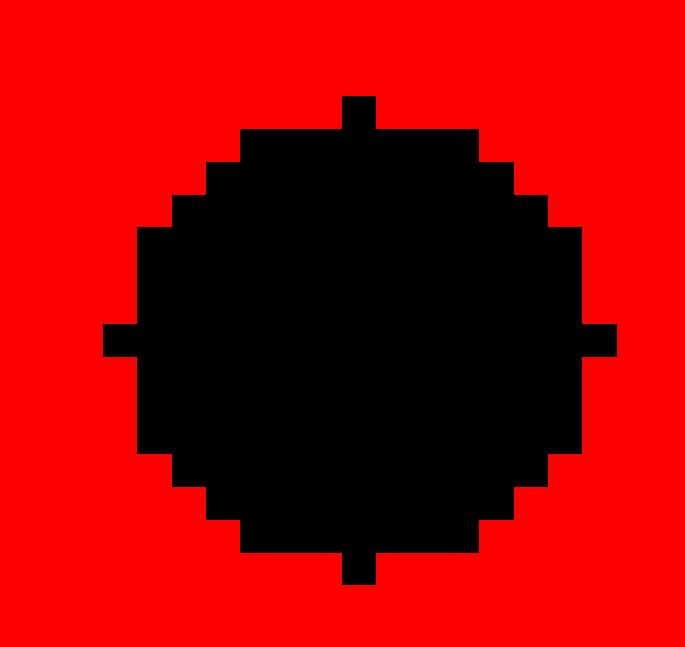
View/Sys/Gal: Ode "NonSmoothExs: ( 1a) plot of step(x)" in "PlottingCurves." This ode is defined by the equation: dx/dt = F. Functions are: F = step(x). This is the unit step function defined as follows: step(x) = 0 if x < 0, step(x) = 1 if x >= 0. The function F has a discontinuity at x = 0 so it is not differentiable at x = 0. The ode is dx/dt = 0 if x < 0, dx/dt = 1 if x >= 0. Solutions are lines parallel to the t axis for x < 0 and parallel lines at 45 degrees for x >= 0. In the phase space x is a fixed point iff x < 0. Image 1: F(x) = step(x) in red, the vector field for dx/dt = step(x). Apply WA to step(x) on [-2,2]
|
|
|
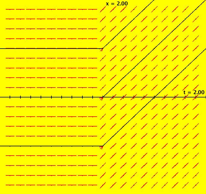
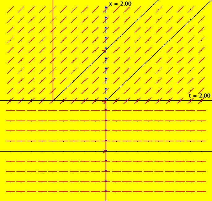
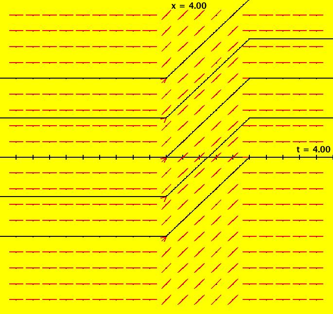
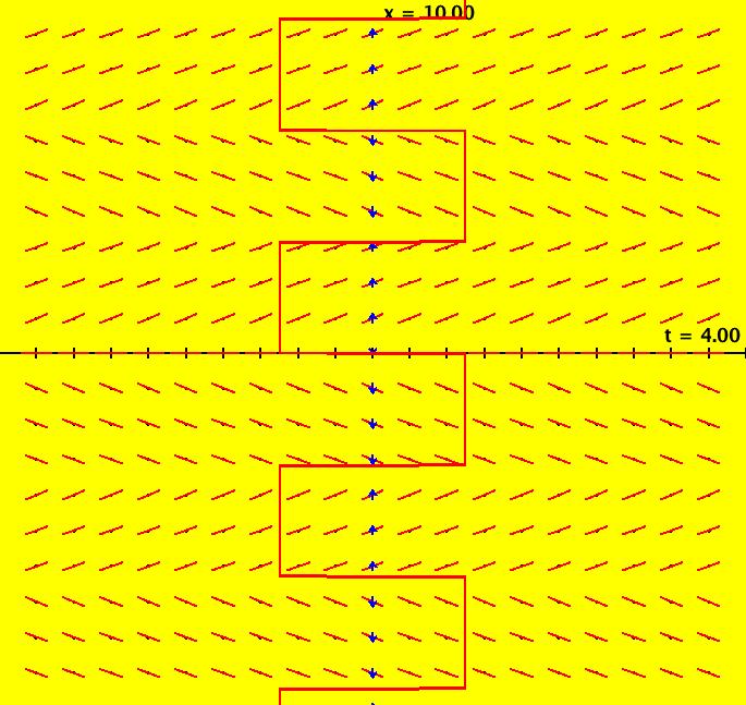
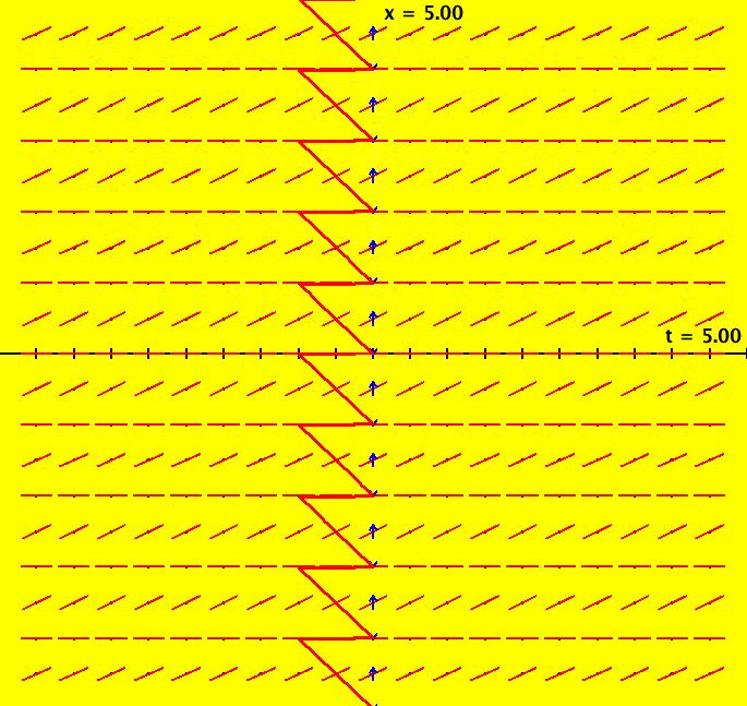
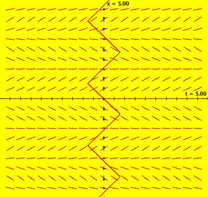
View/Sys/Gal: Ode "NonSmoothExs: ( 1b) dx/dt = step(t)" in "PlottingCurves." This is a nonautonomous system, i.e. the vector field is a function of t. In this case the vector field on the x axis is irrelevant. This ode is defined by the equation: dx/dt = F in the (t,x) coordinate system. Functions are: F = step(t) The ode is dx/dt = 0 of t < 0, dx/dt = 1 if t >= 0. The solution curves to the left of the x axis are straight lines parallel to the t axis and parallel lines at 45 degrees to the right of the x axis. The system has no fixed points. Image 1: The slope field for dx/dt = step(t) shows the effect of the step(t) function but it does not show the step function itself.
|
|
|
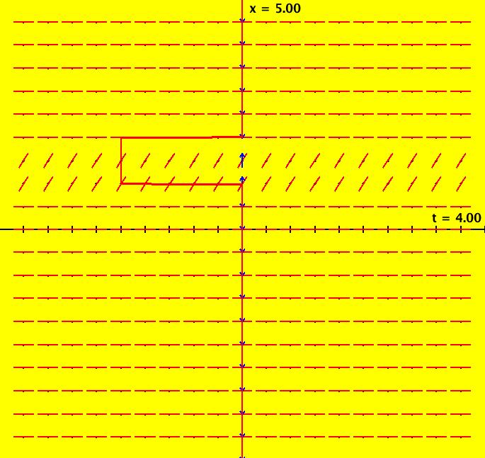
View/Sys/Gal: Ode "NonSmoothExs: ( 2a) plot a*step(x-b), a=1; b=0" in "PlottingCurves." This ode is defined by the equation: dx/dt = F in the (t,x) coordinate system. Parameters are: a=1; b=0 Functions are: F = a*step(x-b) F(x) is the vector field of the autonomous system. Parameter "a" is the amplitude and parameter b shifts the function on the x axis. Image 1: F(x) = 1.5*step(x-.5) in red. Image 2: F(x) = step(x) in red.
|
|
|
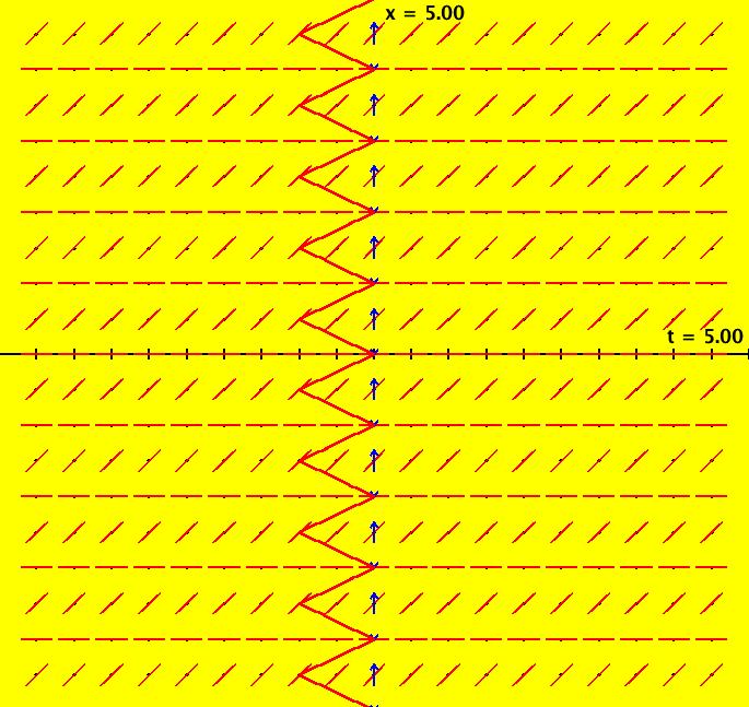
View/Sys/Gal: Ode "NonSmoothExs: ( 2b) a=1; b=0, F = a*step(t-b)" in "PlottingCurves." Note that this is a nonautonomous system so the slope field is shown but the vector field is not shown since it is a function of time. This ode is defined by the equation: dx/dt = F in the (t,x) coordinate system. Parameters are: a=1; b=0 Functions are: F = a*step(t-b) Image 1: The a=1.5, b=.5 case. Image 2: The a=1, b=0, case.
|
|
|
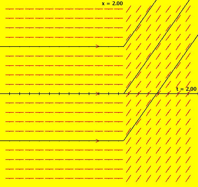
View/Sys/Gal: Ode "NonSmoothExs: ( 3a) a*(step(x-b)-step(x-c)), square pulse function" in "PlottingCurves." For b < c, this is the square pulse function F = a*(step(x-b)-step(x-c)) F = 0 if x < b, = a if b <= x < c and = 0 if x >= c. For a=1, b=0, c=2 the vector field at (2,0) is 0, as it should be, since F = 0 on (- ∞,0) = 1 on [0,2), = 0 on [2,+ ∞). The pulse: height = a = 1, width = c-b = 2, center = (b+c)/2 = 1. Try increasing b, then try increasing c. Image 1: The pulse function of height 2 = a, width 1 = c-b centered at 1.5 = (b+c)/2. So (a,b,c) = (2,1,2). Image 2: The pulse function of height 1 = a, width 2 = c-b centered at 1 = (b+c)/2. So (a,b,c) = (1,0,2). Apply WA to step(x-1)-step(x-3)
|
|
|
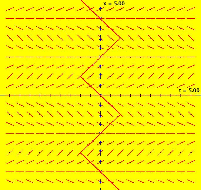
View/Sys/Gal: Ode "NonSmoothExs: ( 3b) a=1; b=0; c=2, F = a*(step(t-b)-step(t-c))" in "PlottingCurves." This is a nonautonomous system. This ode is defined by the equation: dx/dt = F in the (t,x) coordinate system. Parameters are: a=1; b=0; c=2 Functions are: F = a*(step(t-b)-step(t-c)) Image 1: F(t) = a*(step(t-b)-step(t-c)). Slope field.
|
|
|
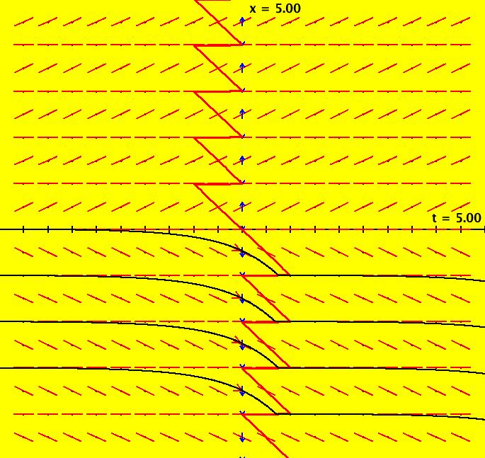
View/Sys/Gal: Ode "NonSmoothExs: ( 4a) x%a, Java remainder or mod function" in "PlottingCurves." The percent sign, %, is called the remainder operator in Java. When written using functional notation, F(x,a) = x%a, it can be thought of as a generalized mod function where x and a are not restricted to positive integers, they can be any int or double. F(x,a) satisfies F(-x,a) = -F(x,a) and F(x,-a) = F(x,a). The definition of F is: F(x,a) = x-n*a on [n*a,(n+1)*a)
where n = 0, 1, ... On the +x axis the graph looks like a sawtooth function with tooth width = height = a. If you rotate the +x graph 180 degrees ccw in the (x,y) plane you get the -x half of the graph, i.e. F(x,a) is an odd function. Image 1: F(x) = x%1 (the vector field) with some solution curves for the autonomous system. Apply WA to (sgn(x)-1)*(a-mod(x,a))/2+(sgn(x)+1)*(mod(x,a)/2) for a=1 The first term is the -x part of the x%a function and the second term is the +x part of the x%a function.
|
|
|
View/Sys/Gal: Ode "NonSmoothExs: ( 4b), a=1, F = t%a" in "PlottingCurves." This is a nonautonomous system. This ode is defined by the equation: dx/dt = F in the (t,x) coordinate system. Parameters are: a=1 Functions are: F = t%a NOTE: User defined functions must always be defined in (t,x,y,z,w) coordinates. Image 1: Some solution curves for the nonautonomous system.
|
|
|
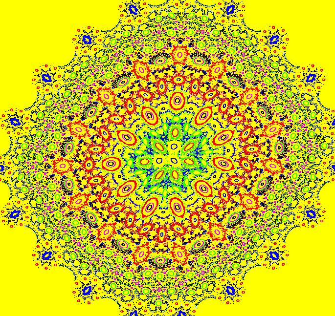
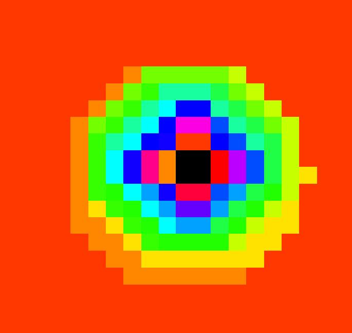
View/Sys/Gal: IMap "NonSmoothExs: ( 4c) (a*b%c), a=23; b=5.5; c=1.5 IMap" in "PlottingCurves." This iteration is defined by: x <- a*b%c. Parameters are: a=23; b=5.5; c=1.5 a*b%c = (a*b)%c = (23*5.5)%1.5 = 126.5%1.5 = .5 So every seed goes to the fixed point x = .5 Image 1: IMap view w/"S On".
|
|
|
View/Sys/Gal: IMap "NonSmoothExs: ( 4d) (a*(b%c)), a=23; b=5.5; c=1.5 IMap" in "PlottingCurves." This iteration is defined by: x <- a*(b%c). Parameters are: a=23; b=5.5; c=1.5 In this case, parentheses have been added to the expression "a*b%c" to force a different evaluation order: a*b%c = (a*b)%c but a*b%c ≠ a*(b%c). (b%c) = 5.5%1.5 = remainder on division by 1.5 = 1 and 23*1 = 23. So, when a*(b%c) is used in place of a*b%c, with the same parameter values, the fixed point changes from .5 to 23. Image 1: IMap view w/"S On"
|
|
|
View/Sys/Gal: IMap "NonSmoothExs: ( 5a) sawtooth or math mod function" in "PlottingCurves." The Java remainder function, combined with the unit step function, can be used to generate the "sawtooth" wave function or the math mod function with period and amplitude "a." F(x) = (sgn(a)+1)/2*(x%a+(1-step(x))*a)- (sgn(a)-1)/2*(x%a+step(x)*a) The sgn factors turn the two terms on and off depending on the sign of parameter "a." Image 1: IMap view, sawtooth wave function for a = -2. Also called the math "mod" function. Image 2: IMap view, sawtooth wave function for a = 1 Apply WA to plot mod(x,a), with a = -2 or to plot x mod a, with a = 1 Note that the Java "mod" operator, %, is NOT the math "mod" function and that the WA "mod" operator, as well as the WA "mod" function IS the math "mod" function.
|
|
|
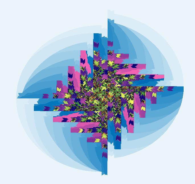
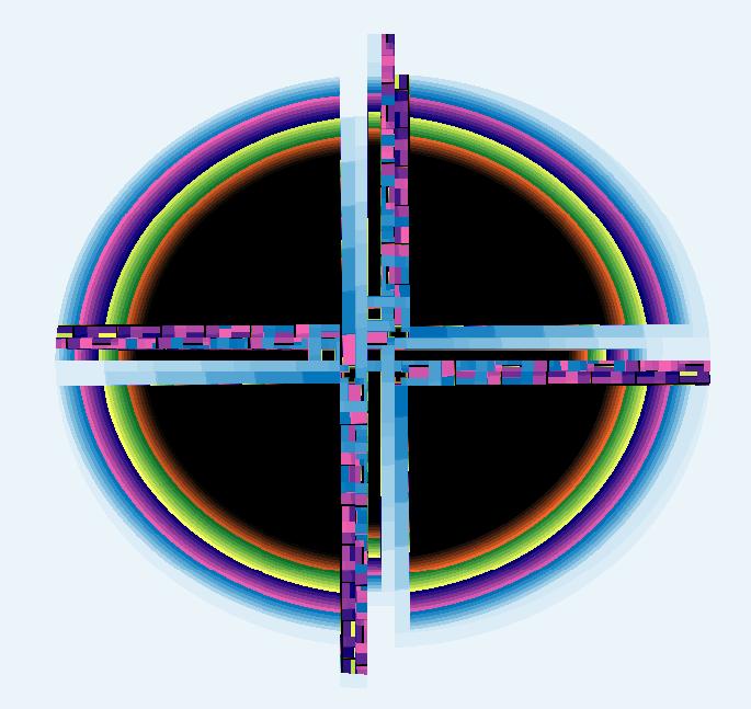
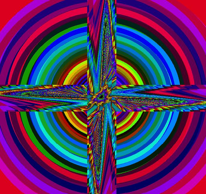
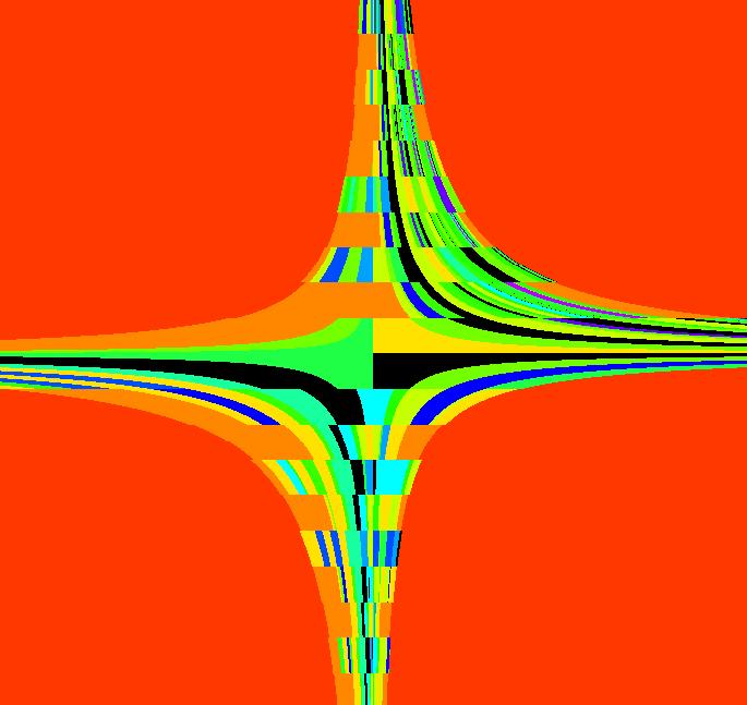
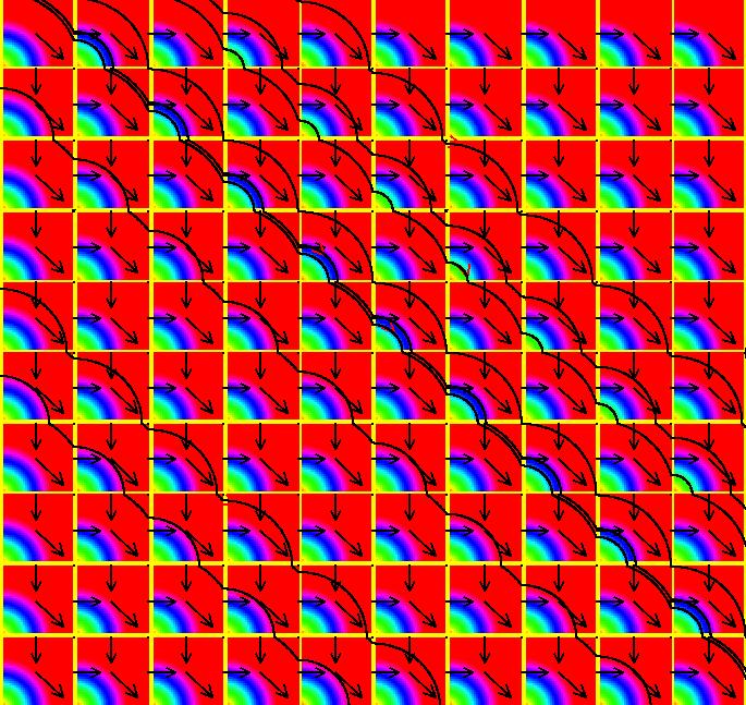
View/Sys/Gal: EMap "NonSmoothExs: ( 5b) EMapCT3" in "PlottingCurves." This iteration is defined by: x <- (1+.1*s)*(y-cos(x%b)), y <- (1+.1*s)*F. Parameters are: a = 6.400; b = 4.800; s = .061; Functions are: F = x%a+(1-step(x))*a EMap CT: 3 Image 1: Nonsmooth functions often produce interesting EMaps.
|
|
|
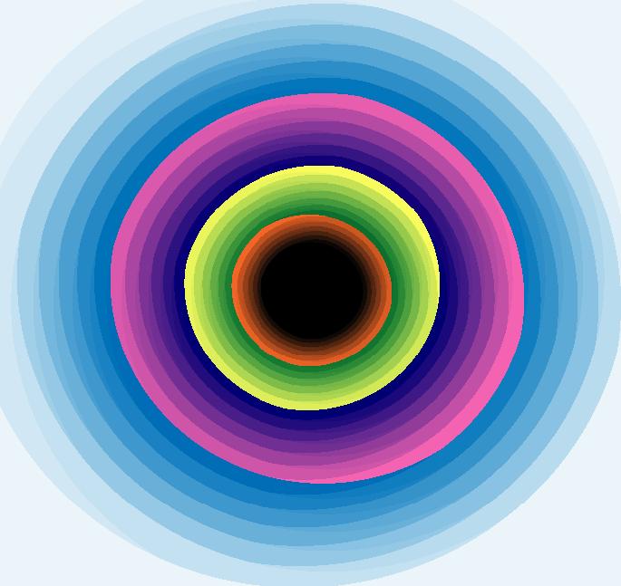
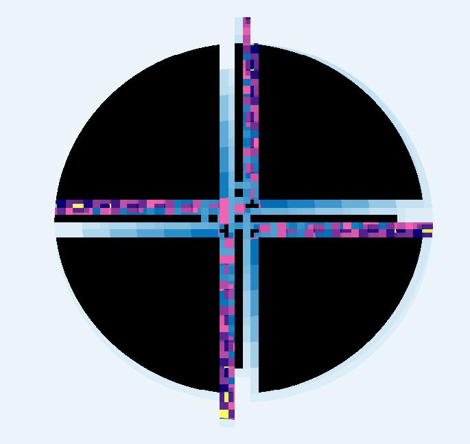
View/Sys/Gal: EMap "NonSmoothExs: ( 5c) EMapCT9 mother and child reunion" in "PlottingCurves." This iteration is defined by: x <- (1+.1*s)*(y-cos(x%b)), y <- (1+.1*s)*F. Parameters are: a = 6.400; b = 4.800; s = .000; Functions are: F = x%a+(1-step(x))*a EMap CT: 9 Image 1: EMap view.
|
|
|
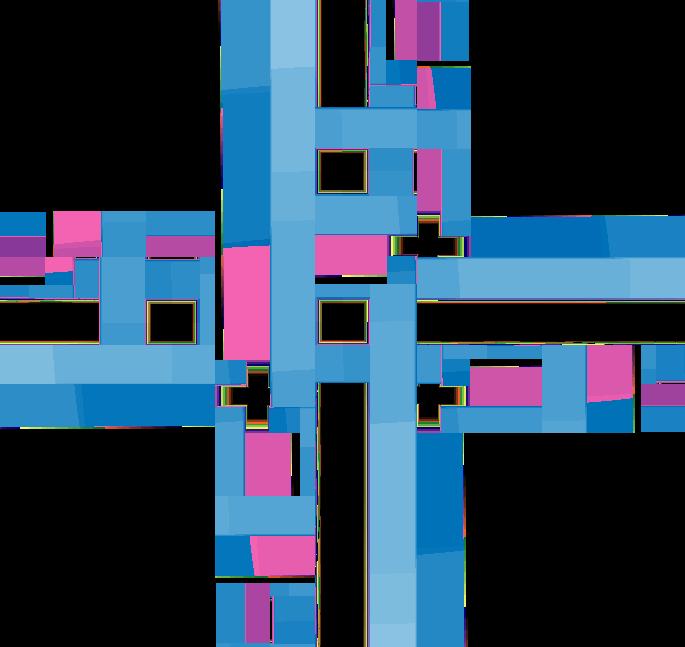
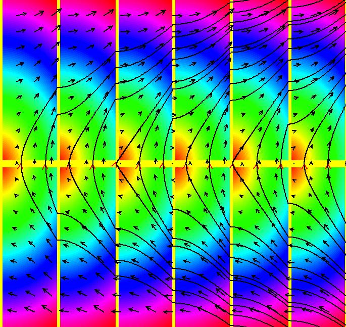
View/Sys/Gal: EMap "NonSmoothExs: ( 5d) using the Java % operator" in "PlottingCurves." This vector field is defined by: V = (y-cos(x%b),F). Parameters are: a = 6.10; b=1 Functions are: F = x%a+(1-step(x))*a Turn the colored vector field. Image 1: The colored vector field in the Ode view. Toggle to the EMap view. Image 2: The EMap view w/CT 0.
|
|
|
View/Sys/Gal: EMap "NonSmoothExs: ( 5e) using the Java % operator" in "PlottingCurves." This vector field is defined by: V = (y-cos(x%b),F) Parameters are: a = -53.00; b = 4.90; Functions are: F = x%a+(1-step(x))*a Turn on the colored vector field. Image 1: The colored vector field in the Ode view zoomed out 2X. The yellow lines are x-nullclines. Toggle to the EMap view. Image 2: The EMap view w/CT 0.
|
|
|
View/Sys/Gal: EMap "NonSmoothExs: ( 5f) EMapCT10" in "PlottingCurves." This iteration is defined by: x <- (1+.1*s)*(y-cos(x%b)), y <- (1+.1*s)*F. Parameters are: a = 6.400; b = 4.800; s = .061; Functions are: F = x%a+(1-step(x))*a EMap CT: 10 Image 1: Yet another EMap. Image 2: EMapMaxCT2.
|
|
|
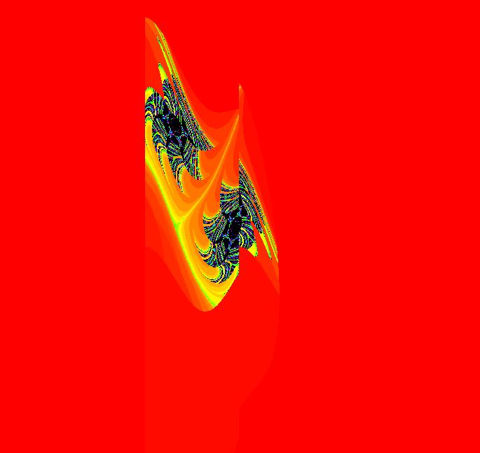
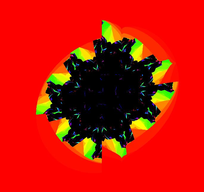
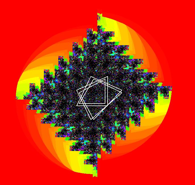
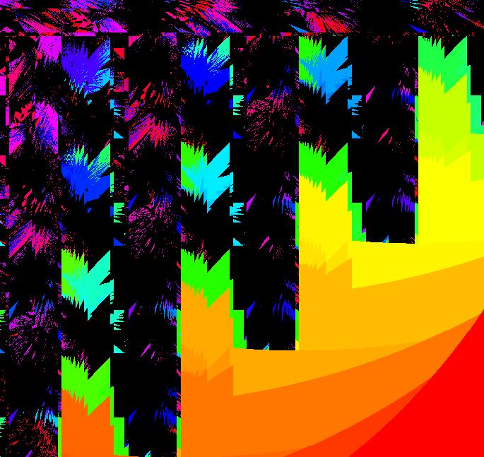
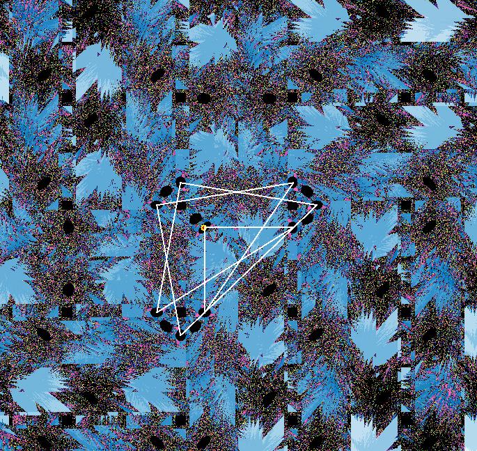
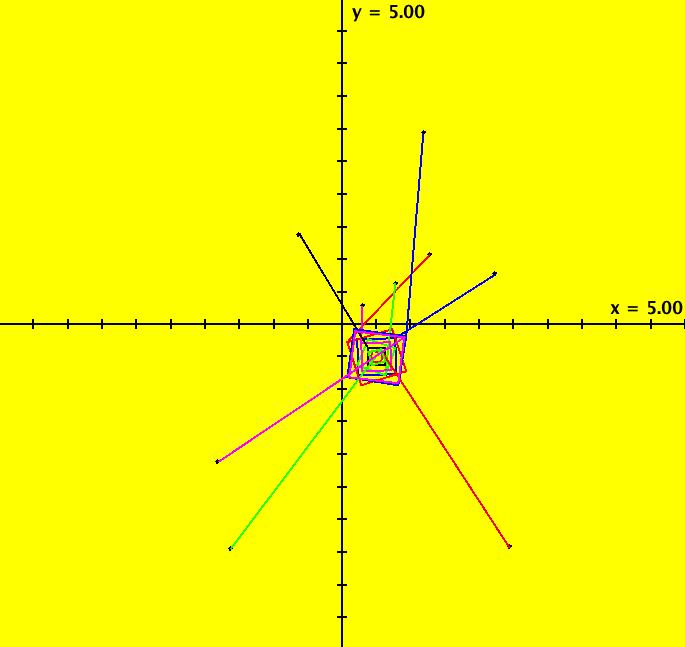
View/Sys/Gal: Ode "NonSmoothExs: ( 6a) using the % operator to create an interesting IMap0011" in "PlottingCurves." This vector field is defined by: Vx = y-sgn(x)*sqrt(abs(b*x-c)), Vy = a-x%d Parameters are: a = .54; b = .43; c = .84; d = 69.00; If you leave out the "%d" factor the system is Barry Martin's well known "hopalong" map from Scientific American September 1986. The parameter values have been chosen at random to give an interesting IMap. Image 1: The IMap0011 view w/31 orbits. You need a lot of orbits to get an interesting image. The "0011" are flag values used to select the IMap display settings on the "Settings" menu. Image 2: The EMap view. There are parts of the EMap to the left and right that are out of the viewing region. Image 3: The Ode view. Only two trajectories are shown. Play with the parameters. You can get back to the original state by selecting the system again. You can save an interesting new version of the system by selecting "Add to Gallery" on the OdeSystem menu. To increase the scale on any of the sliders, move the slider to the edge of the range then close and reopen the parameter controller. To decrease the scale on any of the sliders (to get finer control of the slider position), move the slider to the center of the range then close and reopen the parameter controller. Also try zooming in/out. If you add starting points in either the Ode or IMap view, the new trajectories in the IMap view will not get their new colors until you click the Center button to force a redraw.
|
|
|
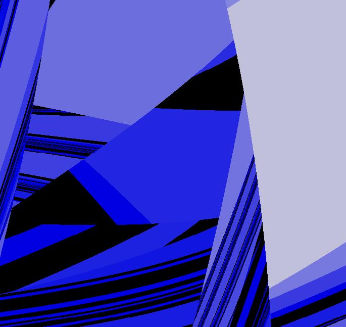
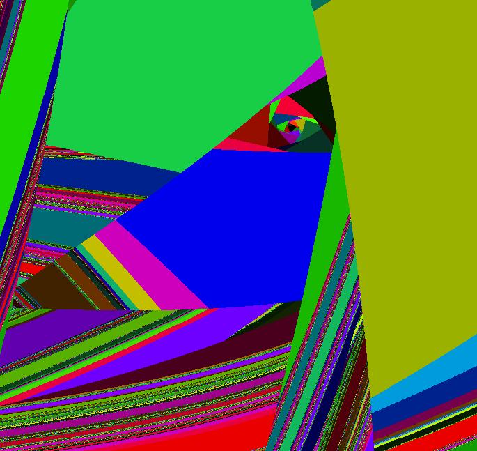
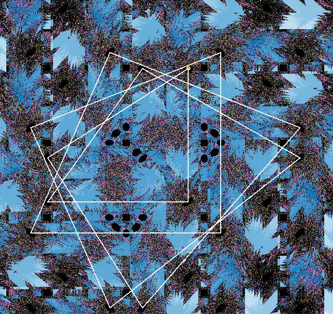
View/Sys/Gal: EMap "NonSmoothExs: ( 6b) variation of (6) as an IMap0011" in "PlottingCurves." This vector field is defined by: Vx = y-sgn(x)*sqrt(abs(b%x-c)), Vy = a-x%d Parameters are: a = -.33; b = .45; c = .86; d = 70.00; Image 1: IMap view with 47 orbits. Some periodic orbits:
|