|

|
View/Sys/Gal: Ode "Lotka-Volterra equations" in "Classic."
Range: (vMax,vMin) = (14.000,-6.000), (hMin,hMax) = (-6.000,14.000)
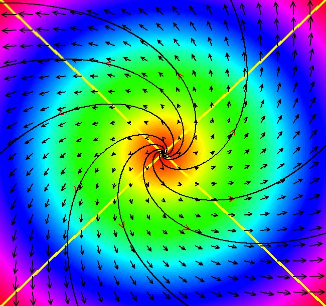
VFld: (-a*x+b*x*y, c*y-d*x*y), a = 1; b = 1; c = 1; d = 1 This system of odes is defined by the equations: dx/dt = -a*x+b*x*y, dy/dt = c*y-d*x*y Parameters are: a = 1; b = 1; c = 1; d = 1 Reference. Mattuck lecture 33. The parameters are all positive and the physical region is the 1st quadrant. It takes 50 minutes but Mattuck proves that the fixed point is a stable center. In WA, enter: plot e^(ln(xy)-x-y), {x,0,5}, {y,0,5} to see the contour curves discussed by Prof. Mattuck. In OdeFactory click the Flow button to see the flow in the phase space. Image 1: Ode trajectories.
ICs | period |
(2,2) | 6.94 |
(3,3) | 8.283 |
(4,4) | 9.94 |
(5,5) | 11.78 |
|

|
View/Sys/Gal: EMap "Lotka-Volterra equations as an EMapCT3" in "Classic."
Range: (vMax,vMin) = (8.062,-1.938), (hMin,hMax) = (-4.962,5.038)
VFld: (-a*x+b*x*y, c*y-d*x*y), a = 1.10; b = 1.50; c = .50; d = .00; This system of odes is defined by the equations: dx/dt = -a*x+b*x*y, dy/dt = c*y-d*x*y Parameters are: a = 1.10; b = 1.50; c = .50; d = .00; Some "art" image examples follow. The images are interesting EMap views of the Lotka-Volterra system created by varying parameters, axis limits and color tables. Image 1: EMap view.
|
|

|
View/Sys/Gal: EMap "Lotka-Volterra equations as an EMapCT3 ver 2" in "Classic."
Range: (vMax,vMin) = (0.016,-0.017), (hMin,hMax) = (-0.015,0.014)
VFld: (-a*x+b*x*y, c*y-d*x*y), a = 1.100; b = 1.000; c = 1.100; d = .000; This iteration is defined by: x <- -a*x+b*x*y, y <- c*y-d*x*y. Parameters are: a = 1.100; b = 1.000; c = 1.100; d = .000; EMap CT: 3 Image 1: Another EMap image.
|
|

|
View/Sys/Gal: EMap "Lotka-Volterra equations as an EMapCT3 ver 3" in "Classic."
Range: (vMax,vMin) = (3.572,-1.428), (hMin,hMax) = (-2.500,2.500)
VFld: (-a*x+b*x*y, c*y-d*x*y), a = 1.100; b = 1.000; c = 1.100; d = 1.000; This iteration is defined by: x <- -a*x+b*x*y, y <- c*y-d*x*y. Parameters are: a = 1.100; b = 1.000; c = 1.100; d = 1.000; EMap CT: 3 Image 1: Yet another EMap image>
|
|

|
View/Sys/Gal: EMap "Lotka-Volterra equations, time scaled as EMap" in "Classic."
Range: (vMax,vMin) = (0.641,-0.641), (hMin,hMax) = (0.478,2.215)
VFld: ((1+s*.01)*(-a*x+b*x*y), (1+s*.01)*(c*y-d*x*y)), a = .90; b = 1.30; c = 1.20; d = .89; s = 4.30; This iteration is defined by: x <- (1+s*.01)*(-a*x+b*x*y), y <- (1+s*.01)*(c*y-d*x*y). Parameters are: a = .90; b = 1.30; c = 1.20; d = .89; s = 4.30; EMap CT: 0 Image 1: Parameter s scales time. Try CT 3. Try zooming out.
|
|

|
View/Sys/Gal: EMap "Lotka-Volterra equations, time scaled as EMapCT3" in "Classic."
Range: (vMax,vMin) = (0.577,0.000), (hMin,hMax) = (1.460,2.271)
VFld: ((1+s*.01)*(-a*x+b*x*y), (1+s*.01)*(c*y-d*x*y)), a = .910; b = 1.000; c = 1.300; d = .890; s = .040; This iteration is defined by: x <- (1+s*.01)*(-a*x+b*x*y), y <- (1+s*.01)*(c*y-d*x*y). Parameters are: a = .910; b = 1.000; c = 1.300; d = .890; s = .040; EMap CT: 3 Image 1: A final EMap image.
|
|

|
View/Sys/Gal: Ode "p. 60, Example 2, from KKO" in "Classic."
Range: (vMax,vMin) = (2.500,-2.500), (hMin,hMax) = (-2.500,2.500)
VFld: (-2*t*x+t) This ode is defined by the equation: dx/dt = -2*t*x+t in the (t,x) coordinate system. The 1st order 1D system corresponds to the 1st order ode y' = -2*x*y+x in the (x,y) coordinate system. This is a 1st order linear, normal ode. It has the standard form: dx/dt+P(t)*x=Q(t). The general solution is: x(t)=1/2+c*e^(-t^2). Image 1: Three solution curves. All solutions go to x = 1/2 as t gets large. All solutions are also symmetric about the t axis. c = 0 gives the straight line through x = 1/2 c = 1 gives the upper curve through x = 3/2 c = -1 gives the lower curve through x = -1/2 This is an example from: "Elementary Differential Equations" by Kreider, Kuller and Ostberg
|
|

|
View/Sys/Gal: Ode "p. 60, Example, from KKO, using fns P and Q" in "Classic."
Range: (vMax,vMin) = (2.560,-2.560), (hMin,hMax) = (-2.560,2.560)
VFld: (-P*x+Q), P = 2*t; Q = t This ode is defined by the equation: dx/dt = -P*x+Q in the (t,x) coordinate system. The 1st order 1D system corresponds to the 1st order ode y' = -P*y+Q in the (x,y) coordinate system. Functions are: P = 2*t; Q = t NOTE: User defined functions must always be defined in (t,x,y,z,w) coordinates. Image 1: Some solution curves. This is an example from: "Elementary Differential Equations" by Kreider, Kuller and Ostberg
|
|


|
View/Sys/Gal: Ode "p. 61, eqn (2-20), from KKO" in "Classic."
Range: (vMax,vMin) = (0.062,-0.062), (hMin,hMax) = (-0.062,0.062)
VFld: (-x/t+1) This ode is defined by the equation: dx/dt = -x/t+1 in the (t,x) coordinate system. The 1st order 1D system corresponds to the 1st order ode y' = -y/x+1 in the (x,y) coordinate system. The general soln is: x(t) = c/t+t/2 for t > 0 and x(t) = -c/t+t/2 for t < 0. c = 0 gives x(t) = t/2 Image 1: Some solution curves. Zoom in to see what is happening near (0,0). Image 2: Image 1 zoomed in. This is an example from: "Elementary Differential Equations" by Kreider, Kuller and Ostberg
|
|

|
View/Sys/Gal: Ode "p. 62, eqn (2-23), from KKO" in "Classic."
Range: (vMax,vMin) = (5.000,-5.000), (hMin,hMax) = (-5.000,5.000)
VFld: (-x+(t*x)^2) Bernoulli's equation has the form: y'+p(x)*y=q(x)*y^n It is nonlinear for all n other than 0 and 1. An example is: dx/dt = -x+(t*x)^2, in (t,x) coordinates, which can also be written in the y(x) form as: y' = -y+(x*y)^2, in (x,y) coordinates In (t,x) coordinates, the solutions are: x(t) = 1/(2+2*t+t^2+c*e^t) and x(t) = 0. Image 1: Solution curves. This is an example from: "Elementary Differential Equations" by Kreider, Kuller and Ostberg
|
|

|
View/Sys/Gal: Ode "p. 64, ex 33, Riccati eqn, from KKO" in "Classic."
Range: (vMax,vMin) = (5.000,-5.000), (hMin,hMax) = (-4.000,6.000)
VFld: ((sin(t)*x)^2-x/(sin(t)*cos(t))-cos(t)^2) This ode is defined by the equation: dx/dt = (sin(t)*x)^2-x/(sin(t)*cos(t))-cos(t)^2 in the (t,x) coordinate system. The 1st order 1D system corresponds to the 1st order ode y' = (sin(x)*y)^2-y/(sin(x)*cos(x))-cos(x)^2 in the (x,y) coordinate system. It is a Riccati equation of the general form: y'+a2(x)*y^2+a1(x)*y+a0(x)=0 A particular soln is: x(t) = cos(t)/sin(t) Image 1: Representative solution curves. This is an example from: "Elementary Differential Equations" by Kreider, Kuller and Ostberg
|
|


|
View/Sys/Gal: Ode "p. 84, eqn (2-52), from KKO" in "Classic."
Range: (vMax,vMin) = (5.000,-5.000), (hMin,hMax) = (-5.000,5.000)
VFld: (y,-(tan(t)-2/tan(t))*y) This system of odes is defined by the equations: dx/dt = y, dy/dt = -(tan(t)-2/tan(t))*y in the (t,x,y) coordinate system. The 1st order 2D system corresponds to the 2nd order ode y'' = -(tan(x)-2/tan(x))*y' in the (x,y,y') coordinate system. Since tan(0) = 0, the 2D system is not defined at t = 0. Image 1: Solution curves in the (t,x) plain with ICs (t,x,y) = (1,1,2) and (-1,1,2). Image 2: Solution curves in the (t,y) plain with ICs (t,x,y) = (1,1,2) and (-1,1,2). This is an example from: "Elementary Differential Equations" by Kreider, Kuller and Ostberg
|
|

|
View/Sys/Gal: Ode "two species competing for the same prey" in "Classic."
Range: (vMax,vMin) = (1.000,-1.000), (hMin,hMax) = (-1.000,1.000)
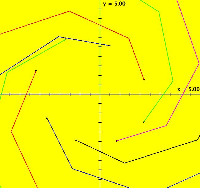
VFld: (x*(1-x)-x*y,2*y*(1-y/2)-3*x*y) This system of odes is defined by the equations: dx/dt = x*(1-x)-x*y, dy/dt = 2*y*(1-y/2)-3*x*y It is a model describing two species competing for the same prey. For more details see; http://www.sosmath.com/diffeq/system/qualitative/qualitative.html Applying WA to 0 = x*(1-x)-x*y, 0 = 2*y*(1-y/2)-3*x*y gives fixed points at (0,2), (.5,.5), (1,0) and (0,0). Image 1: Trajectories in the R2+ view.
|
|

|
View/Sys/Gal: EMap "two species competing for the same prey, EMapCT3 view" in "Classic."
Range: (vMax,vMin) = (0.407,-1.212), (hMin,hMax) = (-0.237,1.222)
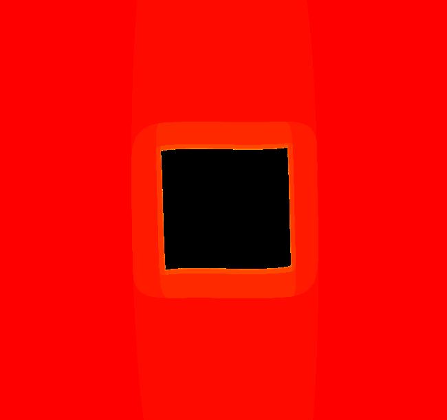
VFld: (x*(c-x)-x*y,a*y*(d-y/2)-b*x*y), a = 1.70; b = 2.10; c = 1.10; d = 1.00; This iteration is defined by: x <- x*(c-x)-x*y, y <- a*y*(d-y/2)-b*x*y. Parameters are: a = 1.70; b = 2.10; c = 1.10; d = 1.00; EMap CT: 3 Image 1: An EMap art image.
|
|

|
View/Sys/Gal: Ode "y'' = (2*y + ln(x))/x^2" in "Classic."
Range: (vMax,vMin) = (5.000,-5.000), (hMin,hMax) = (-5.000,5.000)
VFld: (y, (2*x + ln(t))/t^2) This system of odes is defined by the equations: dx/dt = y, dy/dt = (2*x + ln(t))/t^2 in the (t,x,y) coordinate system. The 1st order 2D system corresponds to the 2nd order ode y'' = (2*y + ln(x))/x^2 in the (x,y,y') coordinate system. The 2D system is not defined at t = 0 and the 2nd order ode is not defined at x = 0. The solution curves in the (t,x) plain can cross because the system is nonautonomous. Image 1: Some x(t) solution curves.
|
|


|
View/Sys/Gal: IMap "y'' = -sin(y)-b*y'+a*cos(c*x)" in "Classic."
Range: (vMax,vMin) = (12.000,-8.000), (hMin,hMax) = (-10.000,10.000)
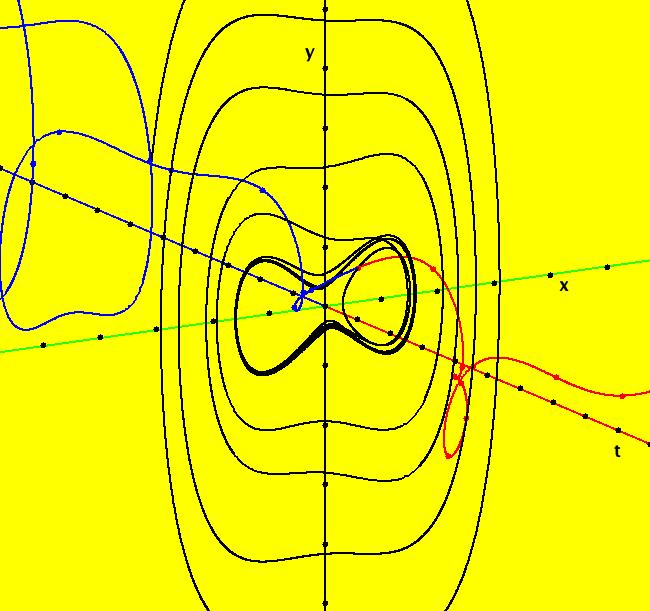
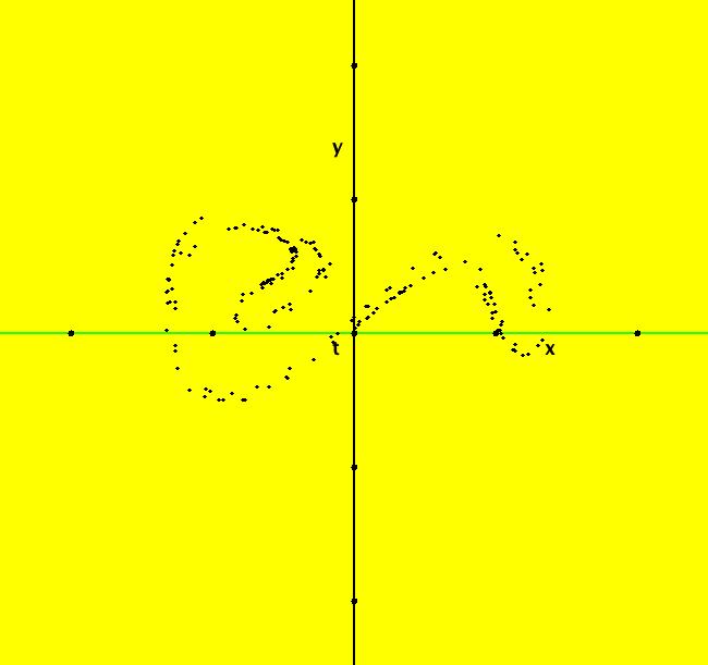
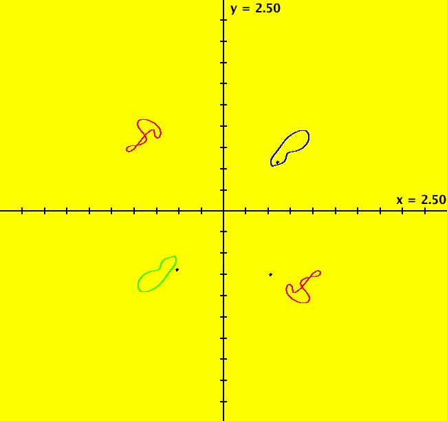
VFld: (y,-sin(x)-b*y+a*cos(c*t)), a = 1.47; b = .5; c = .67 This system of odes is defined by the equations: dx/dt = y, dy/dt = -sin(x)-b*y+a*cos(c*t) in the (t,x,y) coordinate system. The 1st order 2D system corresponds to the 2nd order ode y'' = -sin(y)-b*y'+a*cos(c*x) in the (x,y,y') coordinate system. Parameters are: a = 1.47; b = .5; c = .67 Image 1: Ode view. Image 2: IMap view with blue attractor about (0,0).
|
|


|
View/Sys/Gal: Ode "y'' = 12*x" in "Classic."
Range: (vMax,vMin) = (2.500,-2.500), (hMin,hMax) = (-2.500,2.500)
VFld: (y,12*t) This example comes from "Differential Equations," by Kaj L. Nielsen, p. 23. The problem is to show that: y(x) = 2*x^3 + A*x + B is a solution of the ode: y'' = 12*x, which is easy enough to show. To solve the ode using Ode Factory enter y'' = 12*x in the "y(x) form" field and click "Update Sys" to get: dx/dt = y, (1) dy/dt = 12*t. (2) Integrating (2) gives: y(t) = 6*t^2 + A Using y(t) in (1) and integrating, gives: x(t) = 2*t^3 + A*t + B, To get a particular solution, set A = -2 and B = 0 which corresponds to initial conditions: x(0) = 0, y(0) = -2 The solution curves are: x(t) = 2*t(t^2-1) and y(t) = 2*(3t^2-1) Image 1: x(t). Image 2: y(t). We see that x(t) = 0 at t = -1, 0, 1 and y(t) = 0 at t = sqrt(1/3) = +-0.577. We can plot x vs t and y vs t to verify the solutions. To see that y(t) crosses the t axis at 0.577, click on the crossing point.
|
|


|
View/Sys/Gal: EMap "y'' = x+k*y, k = -2" in "Classic."
Range: (vMax,vMin) = (5.000,-5.000), (hMin,hMax) = (-5.000,5.000)
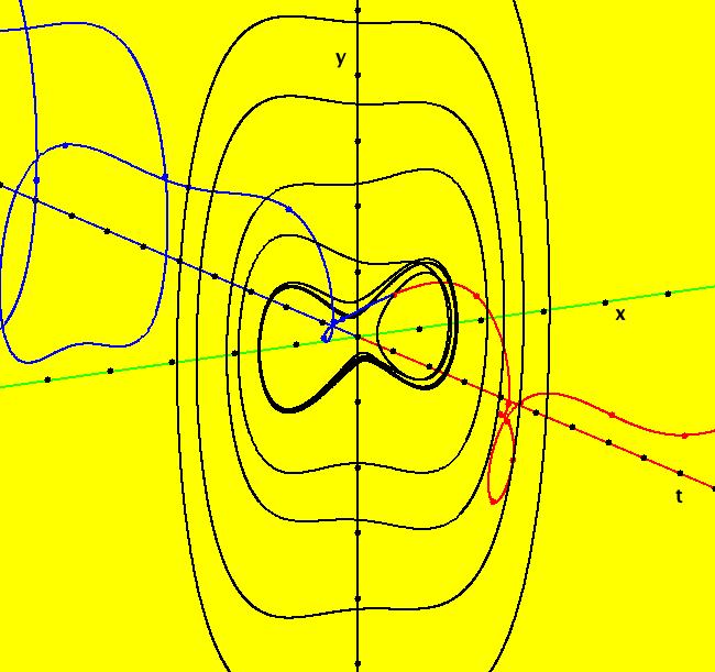
VFld: (y, t+k*x), k = -2 This system of odes is defined by the equations: dx/dt = y, dy/dt = t+k*x in the (t,x,y) coordinate system. The 1st order 2D system corresponds to the 2nd order ode y'' = x+k*y in the (x,y,y') coordinate system. Parameters are: k = -2 Image 1: Ode view. Image 2: EMap view with CT2.
|
|

|
View/Sys/Gal: Ode "y''' = 2*y'' - y' + 2*y +4*x +5*e^(2*x) + 20*cos(x)" in "Classic."
Range: (vMax,vMin) = (5.000,-5.000), (hMin,hMax) = (-5.000,5.000)
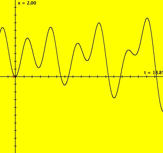
VFld: (y,z, 2*z - y + 2*x +4*t +5*e^(2*t) + 20*cos(t)) This system of odes is defined by the equations: dx/dt = y, dy/dt = z, dz/dt = 2*z - y + 2*x +4*t +5*e^(2*t) + 20*cos(t) in the (t,x,y,z) coordinate system. The 1st order 3D system corresponds to the 3rd order ode y''' = 2*y'' - y' + 2*y +4*x +5*e^(2*x) + 20*cos(x) in the (x,y,y',y'') coordinate system. Image 1: x(1) for y = 2.
|
|

|
View/Sys/Gal: Ode "y'''' = a*y''' +b*y'' + c*y' + d*y" in "Classic."
Range: (vMax,vMin) = (5.000,-5.000), (hMin,hMax) = (-5.000,5.000)
VFld: (y,z,w, a*w +b*z + c*y + d*x), a = 1; b = 2; c = 3; d = 4 This system of odes is defined by the equations: dx/dt = y, dy/dt = z, dz/dt = w, dw/dt = a*w +b*z + c*y + d*x in the (t,x,y,z,w) coordinate system. The 1st order 4D system corresponds to the 4th order ode y'''' = a*y''' +b*y'' + c*y' + d*y in the (x,y,y',y'',y''') coordinate system. Parameters are: a = 1; b = 2; c = 3; d = 4 Image 1: Trajectories in the (x.y) plain for (z,w) = (0,0).
|
|